Class 12 English Important Extra Questions with Answers | English Important Questions Class 12

Class 12 English Important Extra Questions: Here we are providing NCERT Important Extra Questions for Class 12 English Flamingo and Vistas with Answers Pdf Download. Students can get Class 12 English NCERT Solutions, Important Questions of English Class 12 were designed by subject expert teachers.

CBSE NCERT English Class 12 Important Questions with Answers aid students in preparing for their sophomore years start by developing a strong foundation in English subject. This Class 12 English Extra Questions will not only support CBSE Board, UP, MP, Gujarat Board students to score good marks in their internal exams, board exams but also helps to crack the hardest competitive exams like NEET, JEE Main, JEE Advanced, AIIMS, etc. Read on to find out everything regarding CBSE NCERT Extra Questions And Answers for Class 12 English.

English Core Class 12 Important Questions with Answers Pdf Download

Students can check out the Higher Secondary/ 12th Class CBSE NCERT English Important Extra Questions Class 12 subject for all lessons from the quick links provided over here.

Important Questions for Class 12 English Flamingo

Important Questions for Class 12 English Flamingo Prose

  1. The Last Lesson Extra Questions
  2. Lost Spring Extra Questions
  3. Deep Water Extra Questions
  4. The Rattrap Extra Questions
  5. Indigo Extra Questions
  6. Poets and Pancakes Extra Questions
  7. The Interview Extra Questions
  8. Going Places Extra Questions

Important Questions for Class 12 English Flamingo Poetry

  1. My Mother At Sixty-six Extra Questions
  2. An Elementary School Classroom in a Slum Extra Questions
  3. Keeping Quiet Extra Questions
  4. A Thing of Beauty Extra Questions
  5. A Roadside Stand Extra Questions
  6. Aunt Jennifer’s Tigers Extra Questions

Important Questions for Class 12 English Vistas

  1. The Third Level Extra Questions
  2. The Tiger King Extra Questions
  3. Journey to the end of the Earth Extra Questions
  4. The Enemy Extra Questions
  5. Should Wizard hit Mommy Extra Questions
  6. On the face of It Extra Questions
  7. Evans Tries an O-level Extra Questions
  8. Memories of Childhood Extra Questions

We hope the given Chapter Wise Class 12 English Important Extra Questions of Flamingo and Vistas will help you. If you have any queries regarding CBSE English Core Class 12 Important Questions with Answers, drop a comment below and we will get back to you at the earliest.

FAQ’s on Extra Questions for Class 12 English

Question 1.
How to access unit-wise class 12 English extra questions and answers?

Answer:
Just by referring to this page, you all can easily access and collect the unit-wise extra questions for class 12 English for better preparation.

Question 2.
Is there an online portal that provides extra questions for the 12th English board exams?

Answer:
Yes, there are many online portals in this internet world that provide extra questions to prepare effectively and score better marks in the 12th-grade English board exams.

Question 3.
Which is the best website to find the list of class 12 English extra questions?

Answer:
Learninsta.com is the best & trusted website to discover the list of extra questions for 12th class English board exams.

Question 4.
Which question bank is best for the English board exam and includes some extra questions for class 12 English CBSE?

Answer:
Our provided Ncert Solutions for Class 12 English is the best question bank & study material for preparing all the topics included in the 12th English subject. Also, it holds unit-wise extra questions for class 12 English board exams.

Probability Class 12 Notes Maths Chapter 13

By going through these CBSE Class 12 Maths Notes Chapter 13 Probability, students can recall all the concepts quickly.

Probability Notes Class 12 Maths Chapter 13

1. Conditional Probability:
Let E and F be two events with a random experiment. Then, the probability of occurrence of E under the condition that F has already occurred and P(F) ≠ 0 is called the conditional probability. It is denoted by P(E/F).

The conditional probability P(E/F) is given by
P(E/F) = \(\frac{\mathrm{P}(\mathrm{E} \cap \mathrm{F})}{\mathrm{P}(\mathrm{F})}\) , when P(F) ≠ 0.

→ Properties:

  1. 0 ≤ P(E/F) ≤ 1
  2. P(F/F) = 1
  3. P(A ∪ B/F) = P(A/F) + P(B/F) – P(A n B/F)
    If A and B are disjoint events,
    then P(A ∪ B/F) = P(A/F) + P(B/F).
  4. P(E/F) = 1 – P(E/F)

2. Multiplications Probability:
1. Multiplication Theorem on Probability:
Let E and F be two events associated with sample space S. P(E ∩ F) denotes the probability of the event that both E and F occur, which is given by P(E ∩ F) = P(E) P(F/E) = P(F) P(E/F) provided P(E) ≠ 0 and P(F) ≠ 0.
This result is known as the multiplication theorem on probability.

2. Multiplication rule of probability for more than two events:
Let E, F and G be the three events of sample space. Then, P(E ∩F ∩G) = P(E).P(F/E) P[G/(E ∩ F)]

3. Independent Events:

  1. Two events E and F are said to be independent, if P(E/F) = P(E) and P(F/E) = P(F), provided P(E) ≠ 0 and P(F) ≠ 0.
    We know that P(E ∩ F)= P(E). P(F/E) and P(E ∩ F) = P(F). P(E/F).
  2. Events E and F are independent if P(E ∩ F) = P(E) × P(F).
  3. Three events E, F and G are said to be independent or mutually independent, if
    P(E∩F∩G)= P(E). P(F). P(G)

4. Partition of a Sample Space:
A set of events E1, E2,……….., En is said to represent a partition of sample S, if

  1. Ei ∩ Fj = Φ, if i ≠ j, i, j = 1, 2,……….. ,n .
  2. E1 ∪ E2 ∪ E3 ∪ …. ∪ En = S
  3. P(Ei) > 0 for all i = 1, 2,……., n

For example, E and E’ (complement of E) form a partition of sample space S, because
E∩E’ = Φ and E∪E’ = S.

5. Theorem of Total Probability:
Let E1, E2,…….., En be a partition of sample space and each event has a non-zero probability.
If A be any event associated with S, then
P(A) = P(E1) P(A/E1) + P(E2) P(A/E2) + P(E3) P(A/E3) +…….. + P(En) P(A/En)
Probability Class 12 Notes Maths 1
6. Bayes’ Theorem:
Let E1, E2,…………, En be the n events forming a partition of sample space S, i.e., E1, E2,………, E( are pairwise disjoint and E1 ∪ E2 ∪………. ∪
En = S and A is any event of non-zero probability, then
Probability Class 12 Notes Maths 2
7. A Few Terminologies:

  1. Hypothesis: When Bayes’ Theorem is applied, the events E1, E2,……………., En is said to be a hypothesis.
  2. Priori Probability: The probabilities P(E1), P(E2),…………., P(En) is called priori.
  3. Posteriori Probability: The conditional probability P(E./A) is known as the posterior probability of hypothesis E.

8. Random Variable:
A random variable is a real-valued function whose domain is the sample space of a random experiment.
For example, let us consider the experiment of tossing a coin three times.

The sample space of the experiment is
S{TTT, TTH, THT, HTT, HHT, HTH, THH, HHH}

If x denotes the number of heads obtained, then X is the random variable for each outcome.
X(0) = {TTT}
X(1) = {TTH, THT, HTT}
X(2) = {HHT, HTH, THH}
X(3) = {HHH}

9. Probability Distribution of a Random Variable:
Let real numbers x1, x2,…………., xn be the possible values of random variable and p1, p2,……………, pn be probabilities corresponding to each value of the random variable X. Then the probability distribution is
Probability Class 12 Notes Maths 3
It may be noted that

  1. pi > 0
  2. Sum of probabilities p1 + p2 +………….+ pn = 1

Example: Three cards are drawn successively with replacement from a well-shuffled pack of 52 cards. A random variable denotes the number of spades on three cards. Determine the probability distribution of X.
P(S) = P(Drawing a spade) = \(\frac{13}{52}=\frac{1}{4}\)
P(F) = P(Drawing not a space = 1 – \(\frac{1}{4}=\frac{3}{4}\)
P(X = 0) =P(FFF) = \(\left(\frac{3}{4}\right)^{3}=\frac{27}{64}\)
P(X = 1) = 3 × \(\left(\frac{1}{4} \times \frac{3}{4} \times \frac{3}{4}\right)=\frac{27}{64}\)

∵ X = 1 ⇒{SFF, FSF, FFS}
X = 2 ⇒ {SSF, SFS, FSS}
∴ P(X – 2) = 3 × \(\left(\frac{1}{4} \times \frac{1}{4} \times \frac{3}{4}\right)=\frac{9}{64}\)

When X = 3 ⇒ {SSS}
P(X = 3) = \(\frac{1}{4} \times \frac{1}{4} \times \frac{1}{4}=\frac{1}{64}\)
∴ Probability distribution is
Probability Class 12 Notes Maths 4
10. Mean of Random Variable:
Let X be the random variable whose possible values are x1, x2,……….,xn. If p1, p2,……….., pn are the corresponding probabilities, then the mean of X denoted by p is given by
|
The mean of a random variable X is also called the expected value of X, denoted by E(x).
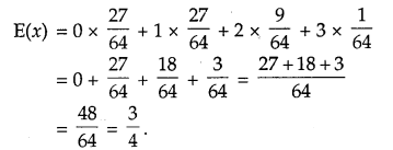
For the experiment of drawing a spade in three cards, the expected value ‘
Probability Class 12 Notes Maths 6
11. Variance of a Random Variable:
Let X be the random variable with possible values of X: x1 x2,……xn occur whose probabilities are p1, p2,………., pn respectively.
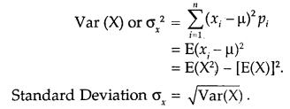
Let μ = E(x) be the mean of X. The variance of X, denoted by Var (X) or σx2, is defined as
Probability Class 12 Notes Maths 7
12. Bernoulli Trial:
Trials of a random experiment are said to be Bernoulli’s Trials if they satisfy the following conditions:

  1. The trials should be independent.
  2. Each trial has exactly two outcomes viz. success or failure.
  3. The probability of success remains the same in each trial.
  4. The number of trials is finite.

Example: An urn contains 6 red and 5 white balls. Four balls are drawn successively. Find whether the trials of drawing balls are Bernoulli trials when after each draw the ball draw is

  1. replaced
  2. not replaced in the urn.

1. If drawing a red ball with replacement is a success, in each trial the probability of success = \(\frac{6}{11}\).
Therefore, drawing a ball with replacement is a Bernoulli trial.

2. In the second attempt, when the ball is not replaced, the probability of success = \(\frac{5}{10}\).

In thired attempt, the probability of success = \(\frac{4}{9}\).
Thus, probability changes at each trial. Hence, in this case, it is not a Bernoulli trial.

13. Binomial Distribution:
The probability distribution of a number of successes in an experiment consisting of n Bernoulli trials is obtained by binomial expansion of (q + p)n.
Such a probability distribution may be written as:
Probability Class 12 Notes Maths 8
This probability distribution is called binomial distribution with parameters n and p.

14. Probability Function:
The probability of x success is denoted by P(x). In a binomial distribution P(x) is given by
P(x) = nCx qn-x px, x = 0,1, 2,…., n and q = 1 – p.
The function P(x) is known as the probability function of the binomial distribution.

1. DEFINITIONS

(i) Random Experiment of Trial. The performance of an experiment is called a trial.
(ii) Event. The possible outcomes of a trial are called events.
(iii) Equally likely Events. The events are said to be equally likely if there is no reason to expect
any one in preference to any other.
(iv ) Exhaustive Events. It is the total number of all possible outcomes of any trial.
(v) Mutually Exclusive Events. Two or more events are said to be mutually exclusive if they
cannot happen simultaneously in a trial. s:
(vi) Favourable Events. The cases which ensure the occurrence of the events are called favourable.
(vii) Sample Space. The set of all possible outcomes of an experiment is called a sample space.
( viii) Probability of occurrences of event A, denoted by P (A), is defined as :
P(A) = \(\frac{\text { No. of favourable cases }}{\text { No. of exhaustive cases }}=\frac{n(\mathrm{~A})}{n(\mathrm{~S})}\)

2. THEOREMS .

(i) In a random experiment, if S be the sample space and A an event, then :
(I) P (A) ≥ 0. (II) P (Φ) = 0 and (III) P (S) = 1.
(ii) If A and B are mutually exclusive events, then P (A ∩ B) = 0.
(iii) If A and B are two mutually exclusive events, then P (A) + P (B) – 1.
(iv) If A and B are mutually exclusive events, then : P (A ∪ B) = P ( A) + P ( B). s
(v) For any two events A and B. P (A ∪ B) = P (A) + P (B) – P (A ∩ B).
(vi) For each event A. P (\(\overline{\mathrm{A}}\)) = 1 – P (A), where (\(\overline{\mathrm{A}}\)) is the complementary event. 1;
( vii) 0 ≤ P (A) ≤ 1.

3. MORE DEFINITIONS
(i) Compound Event. The simultaneous happening of two or more events is called a compound event if they occur in connection with each other. I

(ii) Conditional Probability. Let A and B be two events associated with the same sample spat e then
P (A/B) = \(\frac { No. of elementary events favourable to B which are also favourable to A }{ No. of elementary events favourable to B }\)
Theorem. P (A/B) = \(\frac{P(A \cap B)}{P(B)}\)
P(B/A) = \(\frac{P(A \cap B)}{P(A)}\)

(iii) Independent Events. Two events are said to be independent if the occurrence of one does not a depend upon the occurrence of the other.
Theorem. P (A ∩ B) = P (A) P (B) when A, B are independent.

4. If A1, A1, …………Ar be r events, then the probability when at least one event happens
= 1 – \(\mathbf{P}\left(\overline{\mathbf{A}_{1}}\right) \mathrm{P}\left(\overline{\mathbf{A}_{2}}\right) \ldots \cdot \mathbf{P}\left(\overline{\mathrm{A}}_{r}\right)\)

5. BAYES’ FORMULA
If E1, E2,…., En are mutually exclusive and exhaustive events and A is any event that occurs with E1, E2, …. , En, then :
P(E1/A) = \(\frac{\mathrm{P}\left(\mathrm{E}_{1}\right) \mathrm{P}\left(\mathrm{A} / \mathrm{E}_{1}\right)}{\mathrm{P}\left(\mathrm{E}_{1}\right) \mathrm{P}\left(\mathrm{A} / \mathrm{E}_{1}\right)+\mathrm{P}\left(\mathrm{E}_{2}\right) \mathrm{P}\left(\mathrm{A} / \mathrm{E}_{2}\right)+\ldots \ldots \ldots+\mathrm{P}\left(\mathrm{E}_{n}\right) \mathrm{P}\left(\mathrm{A} / \mathrm{E}_{n}\right)}\)

6. MEAN AND VARIANCE OF RANDOM VARIABLE.
Mean (μ) = Σxipi
Variance (σ2) = Σ(xi – μ)2pi = Σxi2 pi – μ2

Linear Programming Class 12 Notes Maths Chapter 12

By going through these CBSE Class 12 Maths Notes Chapter 12 Linear Programming, students can recall all the concepts quickly.

Linear Programming Notes Class 12 Maths Chapter 12

Linear Programming Problems: Problems that minimize or maximize a linear function Z subject to certain conditions, determined by a set of linear inequalities with non-negative variables, are known as Linear Programming Problems.

Objective Function: A linear function Z = ax + by, where a and b are constants, which has to be maximized or minimized according to a set of given conditions, is called a linear objective function.

Decision Variables: In the objective function Z = ax + by, the variables x, y are said to be decision variables.

Constraints: The restrictions in the form of inequalities on the variables of linear programming problems are called constraints. The conditions x > 0, y > 0 are known as non-negative restrictions.

Example: A dealer deals in only two items: wall hangings and artificial plants. He has ₹ 5,000 to invest in and a space to store at the most 80 pieces. A wall hanging costs him ₹300 and an artificial plant ₹150. He can sell a wall hanging at a profit of ₹50 and an artificial plant at a profit of ₹18. Assuming he can sell all the items that he buys, formulate a linear programming problem in order to maximize his profit.

Let x be the number of wall hanging and y be the number of artificial plants.
Profit on one wall-hanging = ₹50.
∴ Profit by selling x wall hangings = ₹50x
Profit on one artificial plant = ₹18

∴ Profit by selling y artificial plants = ₹18y
The total profit = 50x + 18y
∴ Z = 50x + 18y is the objective function.

A wall hanging costs = ₹300.
∴ Cost of x wall-hangings = ₹300x
The cost of one artificial plant = ₹150

∴ Cost of y artificial plants = ₹150y
The total investment = ₹(300x + 150y)

But the maximum investment = ₹15000
⇒ 300x + 150y ≤ 15000
or
2x + y ≤ 100.

Further, storage capacity to a maximum is 80 pieces.
⇒ x + y ≤ 80.

We know that x ≥ 0, y ≥ 0
Thus, the constraints are 2x + y ≤ 100, x + y ≤ 80,
x ≥ 0, y ≥ 0

Graphical Method of solving a linear programming Problem:
In the above example, the constraints are 2x + y ≤ 100, x + y ≤ 80, x ≥ 0, y ≥ 0.

Now, we draw the lines 2x + y = 100, x + y = 80, x = 0, y = 0 and we find the regions which represent these inequalities.
(i) Consider the inequality
2x + y ≤ 100 .
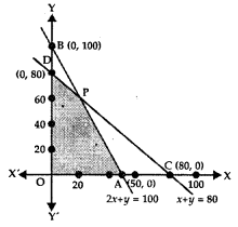
The line 2x + y = 100 passes through A(50, 0) and B(0,100).
Linear Programming Class 12 Notes Maths 1
Putting x = 0, y = 0 in 2x + y ≤ 100, we get 0 ≤ 100, which is true.

This shows origin lies in this region, i.e., the region 2x + y ≤ 100 lies on and below AB as shown in the figure.
1. Next inequality is x + y ≤ 80.
The line x + y = 80 passes through C(80,0) and D(0, 80).
Putting x = 0, y = 0 in x + y < 80, we get 0 ≤ 80, which is true.
⇒ Origin lies in this region, i.e., the region x + y ≤ 80 is on and below CD.
(iii) x > 0 is the region on and to the right of the y-axis.
(iv) y > 0 is the region on and above the x-axis.

→ Feasible Region: The common region determined by all the constraints including non-negative constraints x, y > 0 of linear programming problem is known as feasible region.
In the figure drawn, the shaded area OAPD is the feasible region, which is the common area of the regions drawn under the given constraints.

→ Feasible Solution: Points within and on the boundary of the feasible region represents feasible solutions of constraints.

In the above figure, every point of the shaded area (feasible region) is the feasible solution.
In the feasible region, there are infinitely many points (solutions) that satisfy the given conditions. But we would like to know the points, where Z is maximum or minimum.

→ Theorem 1: Let R be the feasible region for a linear programming problem and let Z = ax + by be the objective function. When Z has an optimum value (maximum or minimum), where variables x and y are subject to constraints described by linear inequalities, the optimal value must occur at a corner point (vertex) of the feasible region.

→ Theorem 2: Let R be the feasible region for a linear programming problem and let Z = ax + by be the objective function. If R is bounded, then the objective function Z has both maximum and minimum value on R and each of these occurs at a corner point (vertex) of R.

Solving the equation 2x + y = 100 and x + y = 80, we get the coordinates of the point P(20, 60). •
In the example given above,
The values of Z at corner points are
At D (0, 80), Z = 50x + 18y = 18 × 80 – 1440
At P(20, 60), Z = 50 × 20 + 18 × 60 = 1000 + 1080 = 2080
At A(50, 0), Z = 50 × 50 + 0 = 2500
At 0(0, 0), Z = O.
Thus, the maximum value of Z is ₹2080 at P(20, 60) and the minimum value of Z is ₹1440 at D(0, 80). In fact, the minimum value is ₹0 at O.

However, if the feasible region is unbounded, the optimal value obtained may not be maximum or minimum.

To determine the optimal point, we proceed as follows:

  1. Let M be the maximum value found as explained above, if the open half-plane determined by ax + by > M has no point in common with the feasible region, then M is the maximum value of Z. Otherwise Z has no maximum value.
  2. Similarly, if m is the minimum value of Z and if the open half-plane determined by ax + by < m, has no point in common with the feasible region, then m is the minimum value of Z, otherwise, Z has no minimum value.

Different Types of Linear Programming Problems:
A few important linear programming problems are as follows:
1. Manufacturing Problem: In such a problem, we determine

  1. a number of units of different products to be produced and sold.
  2. Manpower required, Machine hours needed, warehouse space available, etc. The objective function is to maximize profit.

2. Diet Problem: Here we determine the number of different types of constituents or nutrients which should be included in the diet. The objective function is to minimize the cost of production.

3. Transportation Problems: These problems deal with the costs of transportation which are to be minimized under given constraints.

1. LINEAR PROGRAMMING

Linear programming is a too! which is used in decision making in business for obtaining maximum and minimum values of quantities subject to certain constraints.

2. MATHEMATICAL FORMULATION

Let the linear function Z be defined by :
(i) Z = c1 x1 + c2x2 + … + cnxn, where c’s are constants.
Let aij. be (mn) constants and bj. be a set of m constants such that:
a11x1 + a12 x2 + … + a1n xn (≤ , = ,≥) b1
a21x1 + a22 x2 + … + a2n xn (≤ , = ,≥) b2
………………………………..
………………………………..
am1x1 + am2 x2 + … + amn xn (≤ , = ,≥) bm
and let (iii) x1 ≥ 0, x1 ≥ 0, …, x ≥ 0.

The problem of determining the values of x , x^, …, x which maximizes (or minimizes) Z and satisfying above (ii) is called General Linear Programming Problem (LPP).
Note : In (ii), there may be any sign <. =, or >.

3. SOME DEFINITIONS

A. (i) Objective Function. The linear function Z = ax + by, where a, b are constants, which is to be maximized or minimized is called a linear objective function of LPP.
The variables x and y are called decision variables.

(ii) Constraints. The linear inequalities or inequations or restrictions on the variables of a linear programming problem are called constraints of LPP.
The conditions ,r > 0, y > 0 are called non-negative restrictions of LPP.

(iii) Optimization Problem. A problem, in which it is required to maximize or minimize a linear function (say of two variables x and y) subject to certain constraints, determined by a set of linear inequalities, is called the optimizations problem.

(iv) Solution. The values of x, y which satisfy the constraints of LPP is called the solution of the LPP.

(v) Feasible Solution. Any solution of LPP, which satisfies the non-negative restrictions of
the problem, is called a feasible solution to LPP.

(vi) Optimum Solution. Any feasible solution, which optimizes (minimizes or maximizes) the objective function of LPP is called an optimum solution of the general LPP.

B. (i) Feasible Region. The common region, which is determined by all the constraints including non-negative constraints x, y > 0 of a LPP is called feasible region (or solution region.) The region, other than the feasible one, is called an infeasible region.

(ii) Feasible Solution. The points, which lie on the boundary and within the feasible region, represent the feasible solution of the constraints.
Any part outside the feasible solution is called infeasible solution.

(iii) Optimal (Feasible) Solution. Any point in the feasible region, which gives the optimal value (maximum or minimum) of the objective function, is called optimal solution. These points are infinitely many in number.

Theorem I. Let R be the feasible region (convex polygon) for LPP and Z = ax + by, the objective function.

When Z has an optimal value (max. or min.) where x, y are subject to constraints, this optimal value will occur at a comer point (vertex).

Theorem II. Let R be the feasible region for LPP and Z = ax + by, the objecti ve function. If R is bounded , then the objective function Z has both maximum and minimum values of R and each occurs at a corner point (vertex).

Key Point
When R is unbounded, max. (or min.) value of objective function may not exist. In case it exists, it occurs at a comer point of R.

4. CORNER POINT METHOD

In order to solve a Linear Programming Problem we use Corner Point Method which is as below

Step I. Obtain the feasible region of LPP and determine its comer points (vertices).
Step II. Evaluate the objective function Z = ax + by at each comer point (vertex).
Let M and m be the largest and smallest values at these points.
Step III. (a) When the feasible region is bounded,
then M and m are the maximum and minimum values of Z.

(b) When the feasible region is unbounded, then
(i) M is the maximum value of Z if the open half-plane determined by ax + by > M has no common point with the feasible region; otherwise Z has no maximum value
(ii) m is the minimum value of Z if the open half-plane determined by ax + by < m has no common point with the feasible region; otherwise Z has no minimum value.

Three Dimensional Geometry Class 12 Notes Maths Chapter 11

By going through these CBSE Class 12 Maths Notes Chapter 11 Three Dimensional Geometry, students can recall all the concepts quickly.

Three Dimensional Geometry Notes Class 12 Maths Chapter 11

1. Direction cosines of a line:
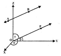
Let AB be a line in space.
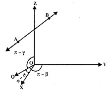
Through O, draw a line OP parallel to AB. Let OP makes angles α, β, and γ with OX, OY, and OZ respectively.
Three Dimensional Geometry Class 12 Notes Maths 1
Cosines of the angles α, β, and γ,
i.e., cos α, cos β, and cos γ are known as the direction cosines of line AB.
Let l = cos α, m = cos β, n = cos γ
⇒ l, m, n are the direction cosines of the line AB Let us consider the ray BA. OQ is drawn parallel to BA. Now, OQ makes angles n – α, n – β, and n – γ with coordinates axes OX, OY, and OZ respectively.
Three Dimensional Geometry Class 12 Notes Maths 2
∴ Direction cosines of BA are cos(π – α), cos (π – β) and cos (π – γ),
i.e., – cos α, – cos β, – cos γ or -l, -m, -n.

→ Relation between l, m, and n
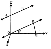
AB is any ray having direction cosines l, m, n. Now OP is drawn parallel to AB, where P is the point (x, y, z). Let PM be drawn perpendicular to OY.
Three Dimensional Geometry Class 12 Notes Maths 3
In ΔOPM OP = r (say). PM⊥OY.
∴ ∠PMO = 90°
Also, ∠POM = β.
∴ \(\frac{\mathrm{OM}}{\mathrm{OP}}\) = β
∴ \(\frac{y}{r}\) = m,
∴ y = rm

Similarly, x = rl and z = rn.
Now, OP2 = x2 + y2 + z2
r2 = (rl)2 + (rm)2 + (rn)2
or
r2 = r2(l2 + m2 + n2)
⇒ l2 + m2 + n2 = 1.

→ Direction Ratios of a line
Definition: The numbers which are proportional to the direction cosines of a line are known as direction ratios of the line.

Let Z, m, n be the direction cosines of a line.
Multiplying each by r, we ger rl, rm, rn the direction ratios.
Let rl = a,rm = b and rn – c.
Squaring and adding
r2l2 + r2m2 + r2n2 = a2 + b2 + c2
∴ r2(l2 + m2 + n2) = a2 + b2 + c2
∵ l2 + m2 + n2 = 1
∴ l = \(\frac{a}{r}=\frac{a}{\sqrt{a^{2}+b^{2}+c^{2}}}\)

Similarly, m = \(\frac{b}{\sqrt{a^{2}+b^{2}+c^{2}}}\) and n = \(\frac{c}{\sqrt{a^{2}+b^{2}+c^{2}}}\)

Thus, if a, b and c are the direction ratios of a line, the direction cosines are \(\frac{a}{\sqrt{a^{2}+b^{2}+c^{2}}}\), \(\frac{b}{\sqrt{a^{2}+b^{2}+c^{2}}}\) and \(\frac{c}{\sqrt{a^{2}+b^{2}+c^{2}}}\).

→ Direction cosines of the line passing through the points P(x1, y1, z1) and Q(x2, y2, z2)
Direction ratios of the line PQ are x2 – x1, y2 – y1, z2 – z1
∴ PQ = \(\sqrt{\left(x_{2}-x_{1}\right)^{2}+\left(y_{2}-y_{1}\right)^{2}+\left(z_{2}-z_{1}\right)^{2}}\)
∴Direction cosines of PQ are \(\frac{x_{2}-x_{1}}{\mathrm{PQ}}\), \(\frac{y_{2}-y_{1}}{\mathrm{PQ}}\), \(\frac{z_{2}-z_{1}}{P Q}\)

2. Angle between the two lines
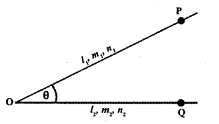
1. Let l1, m1, n1, and l2, m2, n2 be the direction cosines of the lines OP and OQ.
Three Dimensional Geometry Class 12 Notes Maths 4
The angle θ between these lines is given by
cos θ = l1l2 + m1m2 + n1n2
and sin θ = \(\sqrt{\left(m_{1} n_{2}-m_{2} n_{1}\right)^{2}+\left(n_{1} l_{2}-n_{2} l_{1}\right)^{2}+\left(l_{1} m_{2}-l_{2} m_{1}\right)^{2}}\)

2. If a1, b1, c1 and a2, b2, c2 are the direction ratios of two lines, then
Three Dimensional Geometry Class 12 Notes Maths 5
3. Two lines are perpendicular to each other,
if θ = \(\frac{π}{2}\) ⇒ cos θ = cos \(\frac{π}{2}\) = 0
⇒ l1l2 + m1m2 + n1n2 = 0
or
a1a2 + b1b2 + c1c2 = 0

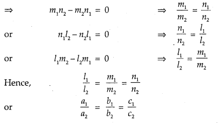
4. When the lines are parallel
θ = 0 ⇒ sin θ = sin 0 = 0.
Three Dimensional Geometry Class 12 Notes Maths 6

STRAIGHT LINE
3. Equation of a line through a given point:
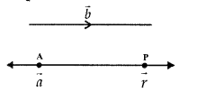
(a) Let the line passes through \(\vec{a}\) and is parallel to vector \(\vec{b}\)
Three Dimensional Geometry Class 12 Notes Maths 7
Then, the equation of the line is
\(\vec{r}\) – \(\vec{a}\) = λ\(\vec{b}\)
or
\(\vec{r}\) = \(\vec{a}\) + λ\(\vec{b}\)

(b) Let the point A be (x1, y1, z1) and a, b, c are the direction ratios of the line. The equation of the line is
\(\frac{x-x_{1}}{a}=\frac{y-y_{1}}{b}=\frac{z-z_{1}}{c}\)
If l, m, n are the direction cosines, then equation of the line is
\(\frac{x-x_{1}}{l}=\frac{y-y_{1}}{m}=\frac{z-z_{1}}{n}\)

4. Equation of the line passing through two points:
(a) Let \(\vec{a}_{1}\), \(\vec{a}_{2}\) be the position vectors of two points P and Q respectively.
⇒ \(\vec{b}\) = \(\vec{a}_{1}\) – \(\vec{a}_{2}\)
Three Dimensional Geometry Class 12 Notes Maths 8
∴ Equation of PQ is
\(\vec{r}\) = \(\vec{a}\) + λ(\(\vec{a}_{2}\) – \(\vec{a}_{1}\))

(b) Direction ratios of the line passing through P(x1, y1, z1) and Q(x2, y2, z2) are x2 – x1, y2 – y1 and z2 – z1
∴ Equation of the line PQ is
\(\frac{x-x_{1}}{x_{2}-x_{1}}=\frac{y-y_{1}}{y_{2}-y_{1}}=\frac{z-z_{1}}{z_{2}-z_{1}}\)

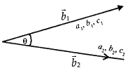
5. Angle between two straight lines:
Three Dimensional Geometry Class 12 Notes Maths 9
(a) Let the two lines be
\(\vec{r}\) = \(\vec{a}_{1}\) + λ\(\vec{b}_{1}\)
\(\vec{r}\) = \(\vec{a}_{2}\) + λ\(\vec{b}_{2}\)
If θ be the angle between them, then
cos θ = \(\frac{\vec{b}_{1} \vec{b}_{2}}{\left|\vec{b}_{1}\right|\left|\vec{b}_{2}\right|}\)

(b) Let the lines be
\(\frac{x-x_{1}}{a_{1}}=\frac{y-y_{1}}{b_{1}}=\frac{z-z_{1}}{c_{1}}\)
and \(\frac{x-x_{2}}{a_{2}}=\frac{y-y_{2}}{b_{2}}=\frac{z-z_{2}}{c_{2}}\)
i.e., a1, b1, c1 and a2, b2, c2 are the direction ratios of the lines.
∴ cos θ = \(\frac{a_{1} a_{2}+b_{1} b_{2}+c_{1} c_{2}}{\sqrt{a_{1}^{2}+b_{1}^{2}+c_{1}^{2}} \sqrt{a_{2}^{2}+b_{2}^{2}+c_{2}^{2}}}\)
If l1, m1, n1 and l2, m2, n2 are the direction cosines, then
cos θ = l1l2 + m1m2 +n1n2

6. Shortest Distance:
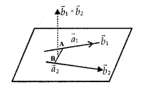
(a)Let \(\vec{r}\) = \(\vec{a}_{1}\) + λ\(\vec{b}_{1}\) and
\(\vec{r}\) = \(\vec{a}_{2}\) + λ\(\vec{b}_{2}\) be the two non-intersecting lines.
The shortest distance between the given lines = \(\left|\frac{\left(\vec{b}_{1} \times \vec{b}_{2}\right) \cdot\left(\vec{a}_{2}-\vec{a}_{1}\right)}{\left|\vec{b}_{1} \times \vec{b}_{2}\right|}\right|\)

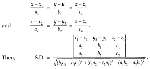
(b) Let the lines be
Three Dimensional Geometry Class 12 Notes Maths 10

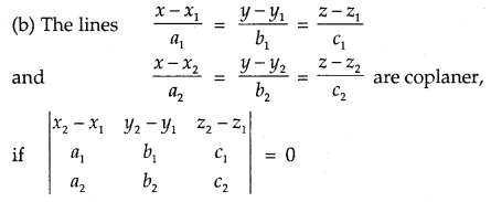
If the lines are intersecting, then lines are coplanar.
⇒ S.D. = 0
⇒ (\(\vec{b}_{1} \times \vec{b}_{2}\)) – (\(\vec{a}_{1} \times \vec{a}_{2}\)) = 0
or
\(\left|\begin{array}{ccc}
x_{2}-x_{1} & y_{2}-y_{1} & z_{2}-z_{1} \\
a_{1} & b_{1} & c_{1} \\
a_{2} & b_{2} & c_{2}
\end{array}\right|\) = 0

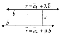
7. Distance between parallel lines:
Let the parallel lines be
\(\vec{r}\) = \(\vec{a}_{1}\) + λ\(\vec{b}_{1}\) and
\(\vec{r}\) = \(\vec{a}_{2}\) + μ\(\vec{b}_{2}\)
Three Dimensional Geometry Class 12 Notes Maths 11
Shortest distance d between these lines is given by,
d = \(\left|\frac{\vec{b} \times\left(\vec{a}_{1}-\vec{a}_{2}\right)}{|\vec{b}|}\right|\)

PLANES
8. Different forms of equations of a plane:
1. Normal Form.
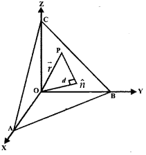
(a) Let the plane ABC be at a distance d from the origin. ON is the normal to the plane in the directon n̂. Equation of the plane is \(\vec{r}\). n̂ = d.
Three Dimensional Geometry Class 12 Notes Maths 12
(b) If l, m, n are the direction cosines of the normal to the plane which is at distance d from the origin. The equation of the plane is lx + my + nz = d.
However, general form of the equation of a plane are \(\vec{r}\) .\(\overrightarrow{\mathrm{N}}\) = D and Ax + By + Cz + D = 0.

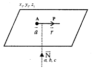
2. (a) Let the plane passes through a point A and let it perpendicular to the vector \(\overrightarrow{\mathrm{N}}\)
∴ Equation of the plane
(\(\vec{r}\) – \(\vec{a}\)).\(\overrightarrow{\mathrm{N}}\) = 0.
Three Dimensional Geometry Class 12 Notes Maths 13

(b) If a plane passes through (x1, y1, z1) and perpendicular to the line with direction ratios a, b, c the equation of the plane is
a(x – x1) + b(y – y1)+c(z – z1) =0

3. Equation of the plane passing through three points.
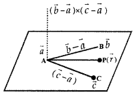
(a) Let the three points be A, B and C whose position vectors be, \(\vec{a}\), \(\vec{b}\) and \(\vec{c}\)
The equation of the plane is
\((\vec{r}-\vec{a}) \cdot[(\vec{b}-\vec{a}) \times(\vec{c}-\vec{a})]\) = 0
Three Dimensional Geometry Class 12 Notes Maths 14
(b) Let the three points through which the plane is passing be A(x1, y1, z1), B(x2, y2, z2), and C(x3, y3, z3).
Then, equation of the plane is
\(\left|\begin{array}{llll}
x & y & z & 1 \\
x_{1} & y_{1} & z_{1} & 1 \\
x_{2} & y_{2} & z_{2} & 1 \\
x_{3} & y_{3} & z_{3} & 1
\end{array}\right|\) = 0
or
\(\left|\begin{array}{ccc}
x-x_{1} & y-y_{1} & z-z_{1} \\
x_{2}-x_{1} & y_{2}-y_{1} & z_{2}-z_{1} \\
x_{3}-x_{1} & y_{3}-y_{1} & z_{3}-z_{1}
\end{array}\right|\) = 0

4. Intercepts form of the equation of the plane
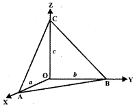
Let the plane make the intercepts a, b, and c on coordinate axes OX, OY, and OZ respectively.
Three Dimensional Geometry Class 12 Notes Maths 15
Then, the equation of the plane is
\(\frac{x}{a}+\frac{y}{b}+\frac{z}{c}\) = 1

9. Plane passing through the intersection of the two planes:
Let the equation of two planes be
\(\vec{r}\). \(\vec{n}_{1}\) = d1 and
\(\vec{r}\) .\(\vec{n}_{2}\) = d2

The equation of the plane passing through the line of intersection of the given planes is
(\(\vec{r}\). \(\vec{n}_{1}\) – d1) + λ(\(\vec{r}\) .\(\vec{n}_{2}\) – d2) = 0
or
\(\vec{r}\) .(\(\vec{n}_{1}\) + λ\(\vec{n}_{2}\)) = (d1 + λd2)

(b) Equation of the plane passing through the line of intersection of the planes
a1x + b1y + c1z + d1 = 0 and a2x + b2y + c2z + d2 = 0 is (a1x + b1 y + c1z + d1 + λ(a2x + b2y + c2z + d2) = 0
or
(a1 + λa2)x + (b1 + λb2)y + (c1 + λc2)z + d1 + λd2 = 0,
where λ is determined according to the given condition.

10. Coplanarity of two lines:
Three Dimensional Geometry Class 12 Notes Maths 16
(a) The two lines
\(\vec{r}\) = \(\vec{a}_{1}\) + λ\(\vec{b}_{1}\) and
\(\vec{r}\) = \(\vec{a}_{2}\) + λ\(\vec{b}_{2}\) intersect each other, if \(\left(\vec{a}_{2}-\vec{a}_{1}\right) \cdot\left(\vec{b}_{2} \times \vec{b}_{1}\right)\) = 0
Three Dimensional Geometry Class 12 Notes Maths 17
11. The angle between the planes:
Definition : The angle between the two planes is the angle between their normals. The angle 0 between the planes
\(\vec{r}\) = \(\vec{n}_{1}\) = d1 and \(\vec{r}\) = \(\vec{n}_{1}\) = d2 is given by cos θ = \(\frac{\left|\vec{n}_{1} \cdot \vec{n}_{2}\right|}{\left|\vec{n}_{1}\right|\left|\vec{n}_{2}\right|}\)

(b) If the planes are
a1x + b1y + C1z + d1 = 0
a2x + b2y + c2z + d2 = 0, then the angle θ between these planes is given by
cos θ = \(\frac{a_{1} a_{2}+b_{1} b_{2}+c_{1} c_{2}}{\sqrt{a_{1}^{2}+b_{1}^{2}+c_{1}^{2}} \sqrt{a_{2}^{2}+b_{2}^{2}+c_{2}^{2}}}\)

(c) The planes are perpendicular to each other, if θ = \(\frac{π}{2}\)
∴ cos \(\frac{π}{2}\) = 0 ⇒ \(\vec{n}_{1}\).\(\vec{n}_{2}\) = 0
or
a1a2 + b1b2 + c1c2 = 0

(d) The planes a1x + b1y +c1z + d1 = 0
and a2x + b2y + c2z + d2 = O
are parallel, if \(\frac{a_{1}}{a_{2}}=\frac{b_{1}}{b_{2}}=\frac{c_{1}}{c_{2}}\).

(e) Equation of the plane parallel to
\(\vec{r} \cdot \vec{n}\) = d is \(\vec{r} \cdot \vec{n}\) = λ
Plane parallel to
ax + by + cz + d = 0 is ax + by + cz + λ = 0.

12. Distance of a point from th plane:
(a) Let the plane be \(\vec{r} \cdot \vec{n}\) = d.
∴ Perpendicular distance of the point \(\vec{a}\) from the plane
=|d – \(\vec{a} \cdot \hat{n}\)|
Three Dimensional Geometry Class 12 Notes Maths 18
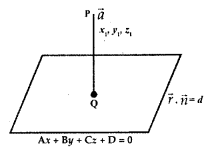
(b) Let the equation of the plane
be Ax + By + Cz + D= O.
The distance of the point (x1, y1, z1) from this plane
= \(\left|\frac{A x_{1}+B y_{1}+C z_{1}+D}{\sqrt{A^{2}+B^{2}+C^{2}}}\right|\)

13. Angle between a line and a plane:
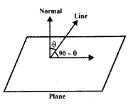
Definition: The angle between a line and plane is said to be the complement of the angle between the line and the normal to the plane.
Three Dimensional Geometry Class 12 Notes Maths 19
(a) Let the line and plane be
\(\vec{r}\) = \(\vec{a}\) + λ\(\vec{b}\) and \(\vec{r} \cdot \vec{n}\) = d.

If θ be the angle between the plane and the line, then
sin θ = \(\frac{\vec{b} \cdot \vec{n}}{|\vec{b}||\vec{n}|}\)

(b) ¡et the line and the plane be \(\frac{x-x_{1}}{a}=\frac{y-y_{1}}{b}=\frac{z-z_{1}}{c}\) and Ax + By + Cz + D = O.
The angle Φ between them is given by
sin Φ = \(\frac{a \cdot \mathrm{A}+b \cdot \mathrm{B}+c \cdot \mathrm{C}}{\sqrt{a^{2}+b^{2}+c^{2}} \sqrt{\mathrm{A}^{2}+\mathrm{B}^{2}+\mathrm{C}^{2}}}\).

1. IMPORTANT RESULT

l2 + m2 + n2 = 1, where < l, m, n > are direction-cosines of a st. line.

2. DIRECTION-RATIOS

The direction-ratios of the line joining of the points (x1, y1, z1) and (x2, y2, z2) are :
<x2-x1, y2-y1 ,z2-z1 >.

3. (i) Angle between two lines. The angle between two lines having direction-cosines
< l1 m1 n1 > and < l2, m2, n2 > is given by :
cos θ = |l1l2+ m1m2 + n1n2|.

(ii) The lines are:
(a) perpendicular l1l2+ m1m2 + n1n2 = 0.
(b) parallel iff l1 = l2, m1 = m2, + n1 = n

4. SHORTEST DISTANCE

The shortest distance between two lines :
\(\vec{r}=\overrightarrow{a_{1}}+\lambda \overrightarrow{b_{1}} \text { and } \vec{r}=\overrightarrow{a_{2}}+\mu \overrightarrow{b_{2}} \text { is }\left|\frac{\left(\overrightarrow{b_{1}} \times \overrightarrow{b_{2}}\right) \cdot\left(\overrightarrow{a_{2}}-\overrightarrow{a_{1}}\right)}{\left|\overrightarrow{b_{1}} \times \overrightarrow{b_{2}}\right|}\right|\)

5. EQUATIONS OF PLANES

(i) Equation of a plane, which is at a distance ‘p’ from the origin and perpendicular to the unit
vector \(\hat{n}\) is \(\vec{r} \cdot \hat{n}=p\)

(ii) General Form. The general equation of first degree i.e.ax + by + cz + d- 0 represents a plane,

(iii) One-point Form. The equation of a plane through (*,, y,, z,) and having <a,b,c> as direction-
ratios of the normal is a (x – x1) + b (y – y1) + c (z – z1) = 0.

(iv) Three-point Form. The equation of the plane through (x1, y1, z1), (x2, y2, z2) and (x3, y3, z3) is:
\(\left|\begin{array}{ccc}
x-x_{1} & y-y_{1} & z-z_{1} \\
x-x_{2} & y-y_{2} & z-z_{2} \\
x-x_{3} & y-y_{3} & z-z_{3}
\end{array}\right|=0\)

(v) Intercept Form. Equation of the plane, which cuts off intercepts a, b, c on the axes, is :
\(\frac{x}{a}+\frac{y}{b}+\frac{z}{c}\) = 1

6. ANGLE BETWEEN TW O PLANES
The angle between the planes :
a1x + b1y + c1z + d1 = 0 and a2x + b2y + c2z + d2 = 0 is given by :
cos θ = \(\frac{\left|a_{1} a_{2}+b_{1} b_{2}+c_{1} c_{2}\right|}{\sqrt{a_{1}^{2}+b_{1}^{2}+c_{1}^{2}} \sqrt{a_{2}^{2}+b_{2}^{2}+c_{2}^{2}}}\)

7. BISECTING PLANES
The equations of the planes bisecting the planes :
a1x + b1y + c1z + d1 = 0 and a2x + b2y + c2z + d2 = 0 are:
\(\frac{a_{1} x+b_{1} y+c_{1} z+d_{1}}{\sqrt{a_{1}^{2}+b_{1}^{2}+c_{1}^{2}}}=\pm \frac{a_{2} x+b_{2} y+c_{2} z+d_{2}}{\sqrt{a_{2}^{2}+b_{2}^{2}+c_{2}^{2}}}\)

Vector Algebra Class 12 Notes Maths Chapter 10

By going through these CBSE Class 12 Maths Notes Chapter 10 Vector Algebra, students can recall all the concepts quickly.

Vector Algebra Notes Class 12 Maths Chapter 10

Some Basic Concepts:
1. Vector (Definition): A quantity that has magnitude, as well as direction, is called a vector.
\(\overrightarrow{\mathrm{AB}}\) is a directed line segment.
Vector Algebra Class 12 Notes Maths 1
It is a vector \(\overrightarrow{\mathrm{AB}}\) and its direction is from A to B.
→ Initial Points: The point A wherefrom the vector \(\overrightarrow{\mathrm{AB}}\) starts is known as the initial point.

→ Terminal point: Point B, where it ends is said to be the terminal point.

→ Magnitude: The distance between initial point and terminal point of a vector is the magnitude (or length) of the vector \(\overrightarrow{\mathrm{AB}}\) . It is denoted by |\(\overrightarrow{\mathrm{AB}}\)| or |\(\overrightarrow{\mathrm{a}}\)| or simply as a.

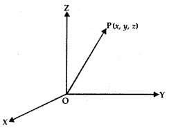
2. Position Vector: Consider a point F(x, y, z) in space. The vector \(\overrightarrow{\mathrm{OP}}\) with an initial point as origin O and terminal point P, is called the position vector of P. It may be denoted by \(\overrightarrow{\mathrm{p}}\).
Vector Algebra Class 12 Notes Maths 2
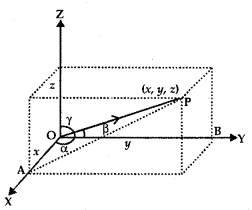
3. Direction Cosines: Let OX, OY, OZ be the coordinates axes and F(x, y, z) be any point in the space. Let OP makes angles α, β, γ with coordinates axes OX, OY, OZ respectively.
Vector Algebra Class 12 Notes Maths 3
The angles α, β, γ are known as direction angles. The cosine of these angles, i.e., cos α, cos β, cos γ is called direction cosines of line OP. These direction cosines are denoted by Z, m, n, i.e., Z = cos α, m = cos β, and n = cos γ.

4. Relation between l, m, n, and Direction Ratios: The perpendiculars PA, PB, PC are drawn on coordinate axes OX, OY, OZ respectively. Let OP = r,
In ΔOAP, ∠A = 90°, cos α = \(\frac{x}{r}\) = l ∴ x = Ir
In ΔABP, ∠B = 90°, cos β = \(\frac{y}{r}\) = m ∴ y = mr
In ΔOCP, ∠C = 90°, cos γ = \(\frac{z}{r}\) = n ∴ z = nr

Thus, the coordinates of P may be expressed as (lr, mr, nr).
Also, OP2 = x2 + y2 + z2 = r2 = (lr)2 + (mr)2 + (nr)2
⇒ l2 + m2 + n2 = 1.
When l, m, n are multiplied by a scalar k, we get the direction ratios, i.e., lk, mk, nk are the direction ratios of OA.

Types of vectors:
1. Zero Vector or Null Vector: A vector whose initial and terminal points coincide is known as zero vector (\(\overrightarrow{0}\)).

2. Unit Vector: A vector whose magnitude is unity is said to be a unit vector. It is denoted as â, so that | â | = 1.

3. Co-initial Vectors: Two or more vectors having the same initial point are called co-initial vectors.

4. Collinear Vectors: If two or more vectors are parallel to the same line, such vectors are known as collinear vectors.

5. Equal Vectors: If two vectors \(\vec{a}\) and \(\vec{b}\) have the same magnitude and direction, regardless of the positions of their initial points, such vectors are said to be equal, i.e., \(\vec{a}\) = \(\vec{b}\) .

6. Negative of a Vector: A vector whose magnitude is the same as that of a given vector (say \(\overrightarrow{\mathrm{AB}}\)), but the direction is opposite to that of it, is known as negative of vector \(\overrightarrow{\mathrm{AB}}\). i.e., \(\overrightarrow{\mathrm{BA}}\) = – \(\overrightarrow{\mathrm{AB}}\).

6. Sum of Vectors:
1. Sum of Vectors \(\vec{a}\) and \(\vec{b}\):
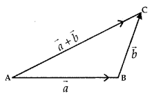
Let the vectors \(\vec{a}\) and \(\vec{b}\) be so positioned that initial point of one coincides with terminal point of the other i.e., let \(\vec{a}\) = \(\overrightarrow{\mathrm{AB}}\) and \(\vec{b}\) = \(\overrightarrow{\mathrm{BA}}\) .
Vector Algebra Class 12 Notes Maths 4
Then, the vector \(\vec{a}+\vec{b}\) is represented by the third side of ΔABC
i. e.,
\(\overrightarrow{\mathrm{AB}}+\overrightarrow{\mathrm{BC}}=\overline{\mathrm{AC}}\) ……..(1)
or
\(\overrightarrow{\mathrm{AC}}+\overrightarrow{\mathrm{AB}}=\overline{\mathrm{BC}}\)
and
\(\overrightarrow{\mathrm{AC}}+\overrightarrow{\mathrm{BC}}=\overline{\mathrm{AB}}\)

This is known as the triangle law of addition.
Further, \(\overrightarrow{\mathrm{AC}}\) = – \(\overrightarrow{\mathrm{CA}}\)
So, (1) may be written as
\(\overrightarrow{\mathrm{AB}}+\overrightarrow{\mathrm{BC}}\) = – \(\overrightarrow{\mathrm{CA}}\)

∴ \(\overrightarrow{\mathrm{AB}}+\overrightarrow{\mathrm{BC}}+\overrightarrow{\mathrm{CA}}\) = \(\overrightarrow{0}\)
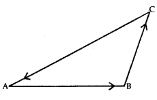
When sides of a triangle ABC are taken in order, i.e., initial and terminal points coincides, then
\(\overrightarrow{\mathrm{AB}}+\overrightarrow{\mathrm{BC}}+\overrightarrow{\mathrm{CA}}\) = \(\overrightarrow{0}\)
Vector Algebra Class 12 Notes Maths 5
2. Parallelogram law of Addition:
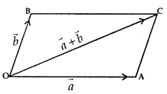
If the two vectors \(\vec{a}\) and \(\vec{b}\) are represented by the two adjacent sides OA and OB of a parallelogram OACB, then their sum \(\vec{a}\) + \(\vec{b}\) is represented in magnitude and direction by the diagonal OC of the parallelogram through their common point O.
Vector Algebra Class 12 Notes Maths 6
i.e., \(\overline{\mathrm{OA}}+\overrightarrow{\mathrm{OB}}=\overrightarrow{\mathrm{OC}}\)

Properties of Vector Addition:
Property 1: For two vectors \(\vec{a}\) and \(\vec{b}\), the sum is commutative i.e.,
\(\vec{a}+\vec{b}\) = \(\vec{b}+\vec{a}\)

Property 2: For three vectors \(\vec{a}\), \(\vec{b}\) and \(\vec{c}\) the sum of vectors is associative,- i.e.,
\((\vec{a}+\vec{b})+\vec{c}\) =\(\vec{a}+(\vec{b}+\vec{c})\)

7. Multiplication of a vector by a scalar:
Let \(\vec{a}\) be the given vector and λ be a scalar.
Product of λ and \(\vec{a}\) = λ\(\vec{a}\).
(i) When λ is +ve, \(\vec{a}\) and λ \(\vec{a}\) have the same sense of direction.
(ii) When λ is -ve, \(\vec{a}\) and λ\(\vec{a}\) are of the opposite directions.
Also, |λ\(\vec{a}\)| = |λ| |\(\vec{a}\)|

→ Additive Inverse of Vector \(\vec{a}\)
If there exists a vector – \(\vec{a}\) such that
\(\vec{a}\) + (- \(\vec{a}\)) = \(\vec{a}\) – \(\vec{a}\) = \(\vec{0}\), then – \(\vec{a}\) is called the additive inverse of \(\vec{a}\).

→ Unit Vector \(\vec{a}\)
Let λ = \(\frac{1}{|\vec{a}|}\) . So, | λ\(\vec{a}\)| = |λ| |\(\vec{a}\)|
= \(\frac{1}{|\vec{a}|}\) × |\(\vec{a}\)| = 1
∴ \(\frac{1}{|\vec{a}|}\) × |\(\vec{a}\)| = a, where |\(\vec{a}\)| ≠ 0 and \(\vec{a}\) is the unit vector.

8. Components of Vector:
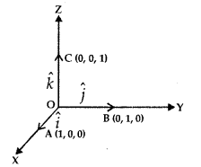
Let us take the points A(1, 0, 0), B(0,1, 0) and 0(0, 0,1) on the co-ordinate axes OX, OY and OZ respectively.
Obviously |\(\overrightarrow{\mathrm{OA}}\)| = 1, |\(\overrightarrow{\mathrm{OB}}\)| = 1 and |\(\overrightarrow{\mathrm{OC}}\)| = 1.

Vectors \(\overrightarrow{\mathrm{OA}}\), \(\overrightarrow{\mathrm{OB}}\) and \(\overrightarrow{\mathrm{OC}}\) each having magnitude 1 are known as unit vectors. They are denoted by î, ĵ and k̂ respectively.
Vector Algebra Class 12 Notes Maths 7
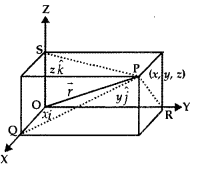
Consider the vector \(\overrightarrow{\mathrm{OP}}\), where P is the point (x, y, z). Now, OQ, OR, OS are the projections of OP on co-ordinates axes.
Vector Algebra Class 12 Notes Maths 8
∴ OQ = x, OR = y, OS = z
\(\overrightarrow{\mathrm{OQ}}\) = xî, \(\overrightarrow{\mathrm{OR}}\) =yĵ, \(\overrightarrow{\mathrm{OS}}\) = zk̂.
⇒ \(\overrightarrow{\mathrm{OP}}\) – xî + yĵ +zk̂.
Also, |\(\overrightarrow{\mathrm{OP}}\)| = \(\sqrt{x^{2}+y^{2}+z^{2}}\) = |\(\vec{r}\)|

x, y, z are called the scalar components and xî, yĵ, and zk̂ are the vector components of vector \(\overrightarrow{\mathrm{OP}}\)

Some properties:
Let \(\vec{a}\) =a1î + a2ĵ + a3k̂ and \(\vec{b}\) =b1î +b2ĵ +b3
1. \(\vec{a}\) + \(\vec{b}\) =(a1 î + a2ĵ + a3k̂) + (b1 î +b2ĵ +b3k̂)
⇒ (a1 + b1)î + (a2 + b2)ĵ + (a3 + b3)k̂

2. \(\vec{a}\) – \(\vec{b}\) or (a1î + a2ĵ +a3k̂) = (b1î + b2ĵ + b3k̂)

3. λ\(\vec{a}\) = λ(a1î + a2ĵ + a3k̂)
⇒ (λa1)î + (λa2)ĵ+ (λa3)k̂

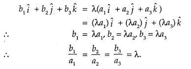
4. \(\vec{a}\) and \(\vec{b}\) are collinear, if and only if there exists a non-zero scalar X such that \(\vec{b}\) = λ\(\vec{a}\), i.e.,
Vector Algebra Class 12 Notes Maths 9
9. Vector joining two points:
Let P1(x1, y1, z1) and P2(x2, y2, z2) be the two points. Then, the vector joining the points P1 and P2 is \(\overline{\mathrm{P}_{1} \mathrm{P}_{2}}\)
Join P1 and P2 with O.
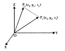
Vector Algebra Class 12 Notes Maths 10
Now,
Vector Algebra Class 12 Notes Maths 11
10. Dividing a line segment in a given ratio:
1. A line segment PQ is divided by a point R in the ratio m: n internally.
Vector Algebra Class 12 Notes Maths 12
i.e., \(\frac{\mathrm{PR}}{\mathrm{RQ}}=\frac{m}{n}\)
If \(\vec{a}\) and \(\vec{b}\) are the position vectors of P and Q then the position vector \(\vec{r}\) of R is given by
\(\vec{r}\) = \(\frac{m \vec{b}+n \vec{a}}{m+n}\)

2. When R divides PQ externally,
\(\frac{\mathrm{PR}}{\mathrm{RQ}}=\frac{m}{n}\)
Vector Algebra Class 12 Notes Maths 13
Replacing n by -n,
\(\vec{r}\) = \(\frac{m \vec{b}-n \vec{a}}{m-n}\)

Product of two vectors (Dot Product)
1. Scalar (or Dot) Product:
Scalar product of two vectors \(\vec{a}\) and \(\vec{b}\) is defined as \(\vec{a}\) . \(\vec{b}\) = | \(\vec{a}\) | \(\vec{b}\) | cos 0, where 0 is the angle between a and b (0,< θ < π).

2. From definition we derive:
(a) \(\vec{a}\).\(\vec{b}\) is a scalar quantity.

(b) When θ = 0, \(\vec{a}\).\(\vec{b}\) = |\(\vec{a}\)| |\(\vec{a}\).\(\vec{b}\)|.
Also, \(\vec{a}\). \(\vec{a}\) = |\(\vec{a}\)|2 = |\(\vec{a}\)|.

(c) When θ = \(\frac{π}{2}\)
⇒ When \(\vec{a}\) ⊥ \(\vec{a}\), \(\vec{a}\). \(\vec{b}\) = 0.

(d) When either \(\vec{a}\) = 0 or \(\vec{b}\) = 0, \(\vec{a}\). \(\vec{b}\) = 0.

(e) cos θ = \(\frac{\vec{a} \cdot \vec{b}}{|\vec{a}||\vec{b}|}\)
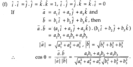
Vector Algebra Class 12 Notes Maths 14
3. Properties of scalar Product
(a) Scalar product is commutative, i.e.,
\(\vec{a}\) . \(\vec{b}\) = \(\vec{b}\).\(\vec{a}\)

(b) If a is scalar, then
(α \(\vec{a}\) ). \(\vec{b}\) = α(\(\vec{a}\).\(\vec{b}\)) – \(\vec{a}\). (α\(\vec{b}\))

11. Projection of vector along a directed line:
Let the vector \(\overrightarrow{\mathrm{AB}}\) makes ar angle θ with directed line l.
Projection of AB on l = |\(\overrightarrow{\mathrm{AB}}\)| cos θ = \(\overrightarrow{\mathrm{AC}}\) = \(\overrightarrow{\mathrm{P}}\).
Vector Algebra Class 12 Notes Maths 15
The vector is \(\overrightarrow{\mathrm{P}}\) is called the projection vector. Its magnitude is
|\(\overrightarrow{\mathrm{P}}\)|, which is known as projection of vector \(\overrightarrow{\mathrm{AB}}\).

The angle θ between \(\overrightarrow{\mathrm{AB}}\) and \(\overrightarrow{\mathrm{AC}}\) is given by
cos θ = \(\frac{\overrightarrow{\mathrm{AB}} \cdot \overrightarrow{\mathrm{AC}}}{|\overline{\mathrm{AB}}||\overline{\mathrm{AC}}|}\)

Now, projection AC = \(\overrightarrow{\mathrm{AB}}\) cos θ = cos θ \(\frac{\overline{\mathrm{AB}} \cdot \overrightarrow{\mathrm{AC}}}{|\mathrm{AC}|}\)
= \(\overrightarrow{\mathrm{AB}}\).(\(\frac{\overrightarrow{\mathrm{AC}}}{|\overrightarrow{\mathrm{AC}}|}\))

If, \(\overrightarrow{\mathrm{AB}}\) = \(\vec{a}\) and \(\overrightarrow{\mathrm{AC}}\) = \(\vec{p}\), then
AC = \(\vec{a}\)(\(\frac{\vec{p}}{|\vec{p}|}\)) = \(\vec{a}\).\(\vec{p}\)

Thus, the projection of \(\vec{a}\) on \(\vec{b}\)
= \(\vec{a}\)(\(\frac{\vec{b}}{|\vec{b}|}\)) = \(\vec{a}\).\(\vec{b}\).

Note: If α, β, γ are the direction angles of the vector
\(\vec{a}\) = (a1î + a2ĵ + a3k̂), the direction cosines of a are given as

cos α = \(\frac{\vec{a} \cdot \hat{i}}{|\vec{a}||\hat{i}|}=\frac{a_{1}}{|\vec{a}|}\)
cos β = \(\frac{a_{2}}{|\vec{a}|}\)
cos γ = \(\frac{a_{3}}{|\vec{a}|}\)

12. Vector Product of two vectors:
1. Definition: The vector product of two non-zero vectors \(\vec{a}\) and \(\vec{b}\), denoted by \(\vec{a}\) × \(\vec{b}\) is defined as
\(\vec{a}\) × \(\vec{b}\) = |\(\vec{a}\) ||\(\vec{b}\) |sin θ.n̂
where θ is the angle between \(\vec{a}\) and \(\vec{b}\), 0 ≤ θ ≤ π. Unit vector n̂ is perpendicular to both vectors \(\vec{a}\) and \(\vec{b}\), such that \(\vec{a}\), \(\vec{b}\) and n̂ form a right handed system.

2. Note:
(a) \(\vec{a}\) × \(\vec{b}\) = | \(\vec{a}\) | | \(\vec{b}\) | sin θ. n̂

  1. If \(\vec{a}\) = 0 or \(\vec{b}\) = 0, \(\vec{a}\) × \(\vec{a}\) = \(\vec{0}\)
  2. \(\vec{a}\) || \(\vec{b}\), \(\vec{a}\) × \(\vec{b}\) = 0

(b) \(\vec{a}\) × \(\vec{b}\) = – \(\vec{b}\) × \(\vec{a}\)
\(\vec{a}\) × \(\vec{b}\) ≠ \(\vec{b}\) × \(\vec{a}\)
⇒ vector product is not commutative.

(c) When θ = \(\frac{π}{2}\), \(\vec{a}\) × \(\vec{b}\) = |\(\vec{a}\)| × |\(\vec{b}\)| × n̂
or
| \(\vec{a}\) × \(\vec{b}\) | = |\(\vec{a}\)||\(\vec{b}\)|

(d) î × î = ĵ × ĵ = k̂ × k̂ = 0
and î × ĵ = k̂, ĵ × k̂ = ĵ, k̂ × î = ĵ.
⇒ĵ × î = – k̂, k̂ × ĵ = -î , î × k̂ = – ĵ.

(e) sin θ = \(\frac{|\vec{a} \times \vec{b}|}{|\vec{a}||\vec{b}|}\)

(f) If \(\vec{a}\) and \(\vec{b}\) represent adjacent sides of a parallelogram, then its area |\(\vec{a}\) × \(\vec{b}\)|.

(g) If \(\vec{a}\) and \(\vec{b}\) represent adjacent sides of a triangle, then its area = \(\frac{1}{2}\) |\(\vec{a}\) × \(\vec{b}\)|

(h) Distributive Property
\(\vec{a}\) × (\(\vec{b}\) + \(\vec{c}\)) = \(\vec{a}\) × \(\vec{b}\) + \(\vec{b}\) x× \(\vec{c}\)
1. Let α be a scalar, then
α(\(\vec{a}\) × \(\vec{b}\)) = (α\(\vec{a}\)) × \(\vec{b}\) = \(\vec{a}\) × (α\(\vec{b}\))

2. \(\vec{a}\) = (a1 î + a2 ĵ + a3 k̂) and
\(\vec{b}\) = (b1 î + b2 ĵ + b3 k̂), then

\(\vec{a}\) × \(\vec{a}\) = \(\left|\begin{array}{lll}
\hat{i} & \hat{j} & \hat{k} \\
a_{1} & a_{2} & a_{3} \\
b_{1} & b_{2} & b_{3}
\end{array}\right|\)

1. PROPERTIES OF \TXHORS UNDER ADDITION

(i) Commutative Law. \(\vec{a}+\vec{b}=\vec{b}+\vec{a}\)
(ii) Associative Law, \(\vec{a}+(\vec{b}+\vec{c})=(\vec{a}+\vec{b})+\vec{c}\)
(iii) Additive Identity. \(\vec{a}+\overrightarrow{0}=\vec{a}=\overrightarrow{0}+\vec{a}\)
(iv) Additive Inverse. \(\vec{a}+(-\vec{a})=\overrightarrow{0}=(-\vec{a})+\vec{a}\)

2. \(\vec{AB}\) = (POSITION VECTOR OF B)-(POSITION VECTOR OF A).

3. SCALAR PRODUCT

(i) Def. The scalar product of \(\vec{a}\) and \(\vec{b}\) is defined as \(\vec{a} \cdot \vec{b}=|\vec{a}||\vec{b}| \cos \theta\), where ‘θ’ is the angle between \(\vec{a}\) and \(\vec{b}\)
(ii) Condition of Perpendicularity. If \(\vec{a}\) and \(\vec{b}\) are perpendicular, then \(\vec{a} \cdot \vec{b}\) = 0.
(iii) If \(\hat{i}, \hat{j}, \hat{k}\) are unit vectors, which are perpendicular to each other, then :
\(\hat{i} \cdot \hat{j}=\hat{j} \cdot \hat{k}=\hat{k} \cdot \hat{i}=0\) and \(\hat{i}^{2}=\hat{j}^{2}=\hat{k^{2}}\)

(iv) Properties:
(a) CommutativeLaw. \(\vec{a}\cdot \vec{b}=\vec{b} \cdot \vec{a}\)

(b) Associative Law, does not hold.

(c) Distributive Laws, \(\vec{a} \cdot(\vec{b}+\vec{c})=\vec{a} \cdot \vec{b}+\vec{a} \cdot \vec{c}\) and \((\vec{b}+\vec{c}) =\vec{b} \cdot \vec{a}+\vec{c} \cdot \vec{a}\)

(d) \((m\vec{a}) \cdot \vec{b}=m(\vec{a} \cdot \vec{b})=\vec{a} \cdot(m \vec{b})\), m being a scalar.

(e) \(\vec{a} \cdot \vec{a}=a^{2}\)

4. VECTOR PRODUCT

(i) Definition. The vector product of \(\vec{a}\) and \(\vec{b}\) is given by: \({a} \times \vec{b}=|\vec{a} \| \vec{b}| \sin \theta \hat{n}\) , where ‘θ’ the angle between \(\vec{a}\) and \(\vec{b}\) and \(\hat{n}\) is a unit vector perpendicular to the plane of \(\vec{a}\) and \(\vec{b}\) .

(ii) When two vectors are parallel, then \(\vec{a} \times \vec{b}=\overrightarrow{0}\)

(iii) If \(\hat{i}, \hat{j}, \hat{k}\) are unit vectors, which are perpendicular to each other, then :
\(\hat{i} \times \hat{j}=\hat{k}=-\hat{j} \times \hat{i} ; \text { etc. } \hat{i} \times \hat{i}=\hat{j} \times \hat{j}=\hat{k} \times \hat{k}=\overrightarrow{0}\)

(iv) Properties :

(a) Commutative Law does not hold.

(b) \((m \vec{a}) \times \vec{b}=m(\vec{a} \times \vec{b})=\vec{a} \times(m b)\), m being a scalar.

(c) If \(\vec{a}=a_{1} \hat{i}+a_{2} \hat{j}+a_{3} \hat{k}, \vec{b}=b_{1} \hat{i}+b_{2} \hat{j}+b_{3} \hat{k}\), then \(\vec{a} \times \vec{b}\) = \(\left|\begin{array}{ccc}
\hat{i} & \hat{j} & \hat{k} \\
a_{1} & a_{2} & a_{3} \\
b_{1} & b_{2} & b_{3}
\end{array}\right|\)

(d) Distributive Law. \(\vec{a} \times(\vec{b}+\vec{c})=\vec{a} \times \vec{b}+\vec{a} \times \vec{c}\)

5. SCALAR TRIPLE PRODUCT

(i) Def. If \(\vec{a}, \vec{b}, \vec{c}\) are three vectors, then the scalar product of \(\vec{a} \times \vec{b}\) with \(\vec{c}\) is called scalar triple product

(ii) Properties:
(a) Condition for three vectors to be coplanar. If \(\vec{a}, \vec{b}, \vec{c}\) are all coplanar vectors, then \(\left[\begin{array}{lll}
\rightarrow & \rightarrow & \rightarrow \\
a & b & c
\end{array}\right]\) = 0

(b) If any two of the three vectors \(\vec{a}, \vec{b}, \vec{c}\) are equal, then \([\vec{a} \vec{b} \vec{c}]\) = 0

(c) If any two of the three vectors \(\vec{a}, \vec{b}, \vec{c}\) are parallel, then \(\left[\begin{array}{ccc}
\rightarrow & \rightarrow & \rightarrow \\
a & b & c
\end{array}\right]\) = 0

(d) In the scalar triple product, the position of dot and cross can be interchanged at pleasure provided the cyclic order of the vectors is maintained.

(e) In the scalar triple product, the change in the cyclic order of die vectors changes the sign of the product.