RS Aggarwal Class 6 Solutions Chapter 8 Algebraic Expressions Ex 8C

RS Aggarwal Class 6 Solutions Chapter 8 Algebraic Expressions Ex 8C

These Solutions are part of RS Aggarwal Solutions Class 6. Here we have given RS Aggarwal Solutions Class 6 Chapter 8 Algebraic Expressions Ex 8C.

Other Exercises

Question 1.
Solution:
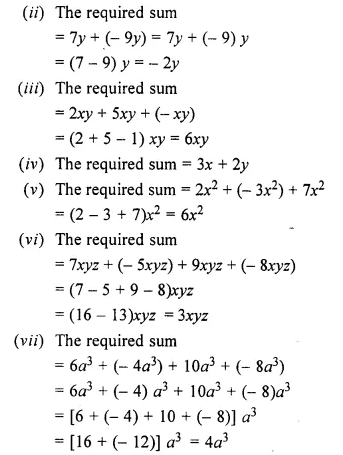
(i) The required sum
= 3x + 7x
= (3 + 7) x
= 10x
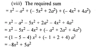
RS Aggarwal Class 6 Solutions Chapter 8 Algebraic Expressions Ex 8C Q1.1
RS Aggarwal Class 6 Solutions Chapter 8 Algebraic Expressions Ex 8C Q1.2

Question 2.
Solution:
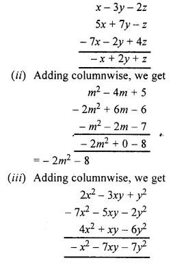
(i) Adding columnwise,
we get
RS Aggarwal Class 6 Solutions Chapter 8 Algebraic Expressions Ex 8C Q2.1
RS Aggarwal Class 6 Solutions Chapter 8 Algebraic Expressions Ex 8C Q2.2

Question 3.
Solution:
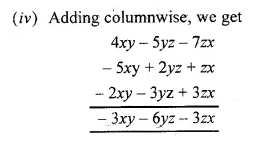
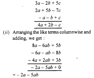
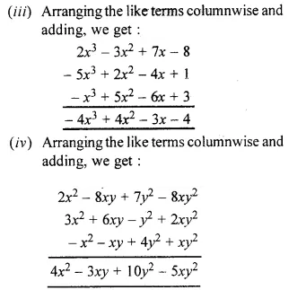
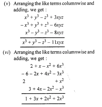
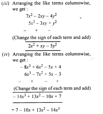
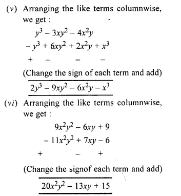
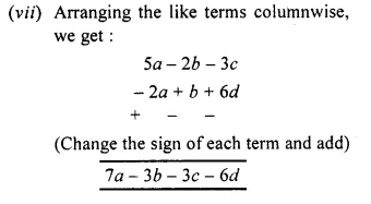
(i) Arranging the like terms columnwise and adding, we get :
RS Aggarwal Class 6 Solutions Chapter 8 Algebraic Expressions Ex 8C Q3.1
RS Aggarwal Class 6 Solutions Chapter 8 Algebraic Expressions Ex 8C Q3.2
RS Aggarwal Class 6 Solutions Chapter 8 Algebraic Expressions Ex 8C Q3.3

Question 4.
Solution:
(i) We have :
2x – 5x = (2 – 5)x = – 3x
(ii) We have :
6x – y – (- xy) = 6xy + xy = 7xy
(iii) We have : 5b – 3a
(iv) We have : 9y – ( – 7x) = 9y + 7x
(v) We have : – 7x2 – 10x2 = ( – 7 – 10)x2
= – 17x2
(vi) We have : b2 – a2 – (a2 – b2)
= b2 – a2 – a2 + b2
= b2 + b2 – a2 – a2
= (1 + 1) b2 + ( – 1 – 1) a2
= 2b2 – 2a2

Question 5.
Solution:
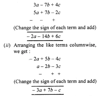
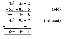
(i) Arranging the like terms columnwise, we get :
RS Aggarwal Class 6 Solutions Chapter 8 Algebraic Expressions Ex 8C Q5.1
RS Aggarwal Class 6 Solutions Chapter 8 Algebraic Expressions Ex 8C Q5.2
RS Aggarwal Class 6 Solutions Chapter 8 Algebraic Expressions Ex 8C Q5.3
RS Aggarwal Class 6 Solutions Chapter 8 Algebraic Expressions Ex 8C Q5.4

Question 6.
Solution:
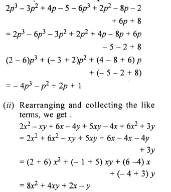
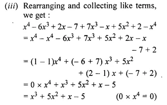
(i) Rearranging and collecting the like terms, we get :
RS Aggarwal Class 6 Solutions Chapter 8 Algebraic Expressions Ex 8C Q6.1
RS Aggarwal Class 6 Solutions Chapter 8 Algebraic Expressions Ex 8C Q6.2

Question 7.
Solution:
We have:
RS Aggarwal Class 6 Solutions Chapter 8 Algebraic Expressions Ex 8C Q7.1

Question 8.
Solution:
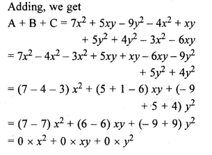
We have :
A = 7x2 + 5xy – 9y2
B = – 4x2 + xy + 5y2
C = 4y2 – 3x2 – 6xy
RS Aggarwal Class 6 Solutions Chapter 8 Algebraic Expressions Ex 8C Q8.1
= 0+0+0 = 0
Hence the result

Question 9.
Solution:
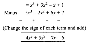
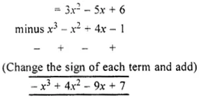
Required expression
RS Aggarwal Class 6 Solutions Chapter 8 Algebraic Expressions Ex 8C Q9.1

Question 10.
Solution:
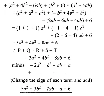
Substituting the values of P, Q, R and S, we have :
P + Q + R + S = (a2 – b2 + 2ab)
RS Aggarwal Class 6 Solutions Chapter 8 Algebraic Expressions Ex 8C Q10.1

Question 11.
Solution:
Required expression
RS Aggarwal Class 6 Solutions Chapter 8 Algebraic Expressions Ex 8C Q11.1

Question 12.
Solution:
Required expression
RS Aggarwal Class 6 Solutions Chapter 8 Algebraic Expressions Ex 8C Q12.1

Question 13.
Solution:
Required expression
RS Aggarwal Class 6 Solutions Chapter 8 Algebraic Expressions Ex 8C Q13.1

Question 14.
Solution:
Required expression
RS Aggarwal Class 6 Solutions Chapter 8 Algebraic Expressions Ex 8C Q14.1

Question 15.
Solution:
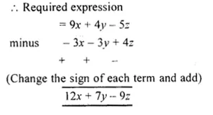
Sum of 5x – 4y + 6z and – 8x + y – 2z
= 5x – 4y + 6z – 8x + y – 2z
= 5x – 8x – 4y + y + 6z – 2z
= – 3x – 3y + 4z
Sum of 12x – y + 3z and – 3x + 5y – 8z
= 12x – y + 3z – 3x + 5y – 8z
= 12x – 3x – y + 5y + 3z – 8z
= 9x + 4y – 5z
RS Aggarwal Class 6 Solutions Chapter 8 Algebraic Expressions Ex 8C Q15.1

Question 16.
Solution:
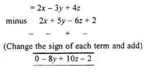
Required expression
RS Aggarwal Class 6 Solutions Chapter 8 Algebraic Expressions Ex 8C Q16.1

Question 17.
Solution:
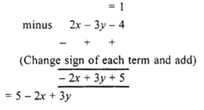
Required expression
RS Aggarwal Class 6 Solutions Chapter 8 Algebraic Expressions Ex 8C Q17.1

Hope given RS Aggarwal Solutions Class 6 Chapter 8 Algebraic Expressions Ex 8C are helpful to complete your math homework.

If you have any doubts, please comment below. Learn Insta try to provide online math tutoring for you.

RS Aggarwal Class 6 Solutions Chapter 10 Ratio, Proportion and Unitary Method Ex 10A

RS Aggarwal Class 6 Solutions Chapter 10 Ratio, Proportion and Unitary Method Ex 10A

These Solutions are part of RS Aggarwal Solutions Class 6. Here we have given RS Aggarwal Solutions Class 6 Chapter 10 Ratio, Proportion and Unitary Method Ex 10A.

Other Exercises

Question 1.
Solution:
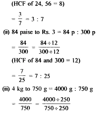
(i) 24 to 56
= \(\\ \frac { 24 }{ 56 } \)
= \(\frac { 24\div 8 }{ 56\div 8 } \)
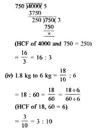
RS Aggarwal Class 6 Solutions Chapter 10 Ratio, Proportion and Unitary Method Ex 10A Q1.1
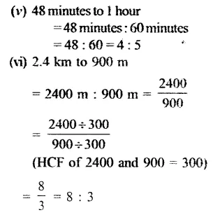
RS Aggarwal Class 6 Solutions Chapter 10 Ratio, Proportion and Unitary Method Ex 10A Q1.2
RS Aggarwal Class 6 Solutions Chapter 10 Ratio, Proportion and Unitary Method Ex 10A Q1.3

Question 2.
Solution:
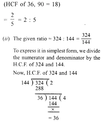
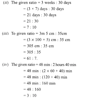
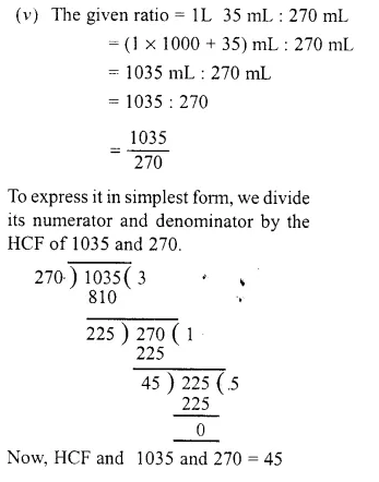
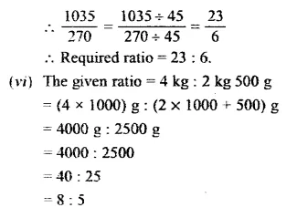
(i) 36 : 90
= \(\\ \frac { 36 }{ 90 } \)
= \(\frac { 36\div 18 }{ 90\div 18 } \)
RS Aggarwal Class 6 Solutions Chapter 10 Ratio, Proportion and Unitary Method Ex 10A Q2.1
RS Aggarwal Class 6 Solutions Chapter 10 Ratio, Proportion and Unitary Method Ex 10A Q2.2
RS Aggarwal Class 6 Solutions Chapter 10 Ratio, Proportion and Unitary Method Ex 10A Q2.3
RS Aggarwal Class 6 Solutions Chapter 10 Ratio, Proportion and Unitary Method Ex 10A Q2.4
RS Aggarwal Class 6 Solutions Chapter 10 Ratio, Proportion and Unitary Method Ex 10A Q2.5

Question 3.
Solution:
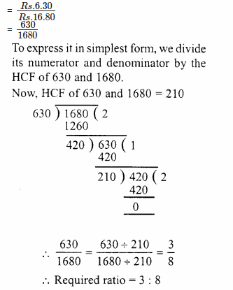
(i) The given ratio = Rs. 6.30 : Rs. 16.80
= \(\\ \frac { Rs.6.30 }{ Rs.16.80 } \)
= \(\\ \frac { 630 }{ 1680 } \)
RS Aggarwal Class 6 Solutions Chapter 10 Ratio, Proportion and Unitary Method Ex 10A Q3.1
RS Aggarwal Class 6 Solutions Chapter 10 Ratio, Proportion and Unitary Method Ex 10A Q3.2
RS Aggarwal Class 6 Solutions Chapter 10 Ratio, Proportion and Unitary Method Ex 10A Q3.3
RS Aggarwal Class 6 Solutions Chapter 10 Ratio, Proportion and Unitary Method Ex 10A Q3.4

Question 4.
Solution:
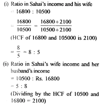
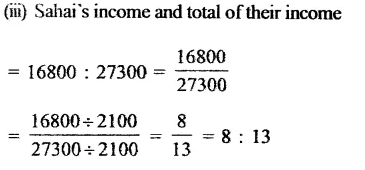
Earning of Sahai = Rs. 16800
and of his wife = Rs. 10500
Then total income = Rs. 16800 + 10500
= Rs. 27300
RS Aggarwal Class 6 Solutions Chapter 10 Ratio, Proportion and Unitary Method Ex 10A Q4.1
RS Aggarwal Class 6 Solutions Chapter 10 Ratio, Proportion and Unitary Method Ex 10A Q4.2

Question 5.
Solution:
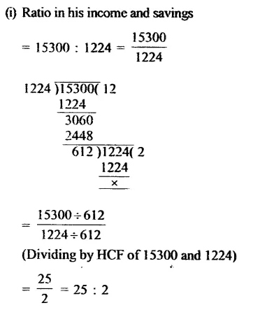
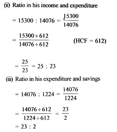
Rohit monthly earnings = Rs. 15300
and his savings = Rs. 1224
So, his expenditure = Rs. 15300 – 1224
= Rs. 14076
Now,
RS Aggarwal Class 6 Solutions Chapter 10 Ratio, Proportion and Unitary Method Ex 10A Q5.1
RS Aggarwal Class 6 Solutions Chapter 10 Ratio, Proportion and Unitary Method Ex 10A Q5.2

Question 6.
Solution:
Let the number of male and female workers in the mill be 5x and 3x respectively. Then,
5x = 115
=> \(\\ \frac { 5x }{ 5 } \) = \(\\ \frac { 115 }{ 5 } \)
(Dividing both sides by 5)
=> x = 23
Number of female workers in the mill
= 3x
= 3 x 23 = 69.

Question 7.
Solution:
Let the number of boys and girls in the school be 9x and 5x respectively.
According to the question,
9x + 5x = 44
=> 14x = 448
=> \(\\ \frac { 14x }{ 14 } \) = \(\\ \frac { 448 }{ 14 } \)
(Dividing both sides by 14)
=> x = 32.
Number of girls =5x
= 5 x 32
= 160

Question 8.
Solution:
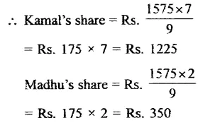
Total amount = Rs. 1575
Ratio in Kamal and Madhu’s share = 7 : 2
Sum of ratios = 7 + 2 = 9
RS Aggarwal Class 6 Solutions Chapter 10 Ratio, Proportion and Unitary Method Ex 10A Q8.1

Question 9.
Solution:
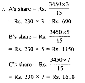
Total amount = Rs. 3450
Ratio in A, B and C shares = 3 : 5 : 7
Sum of share = 3 + 5 + 7 = 15
RS Aggarwal Class 6 Solutions Chapter 10 Ratio, Proportion and Unitary Method Ex 10A Q9.1

Question 10.
Solution:
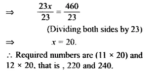
Let the numbers be 11x and 12x.
Then. 11x + 12x = 460
=> 23x = 460
RS Aggarwal Class 6 Solutions Chapter 10 Ratio, Proportion and Unitary Method Ex 10A Q10.1

Question 11.
Solution:
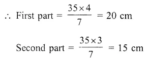
Length of line segment = 35 cm
Ratio = 4 : 3
Sum of ratio = 4 + 3 = 7
RS Aggarwal Class 6 Solutions Chapter 10 Ratio, Proportion and Unitary Method Ex 10A Q11.1

Question 12.
Solution:
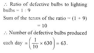
Total bulbs produced per day = 630
Out of every 10 bulbs, defective bulb = 1
Out of every 10 bulbs, lighting bulbs = 10 – 1 = 9
RS Aggarwal Class 6 Solutions Chapter 10 Ratio, Proportion and Unitary Method Ex 10A Q12.1

Question 13.
Solution:
Price of 20 pencils = Rs. 96
(1 score = 20 pencils)
Price of 1 pencil = Rs. (96 ÷ 20)
= Rs. 4.80
Price of 12 ball pens = Rs. 50.40
(1 dozen = 12)
Price of 1 ball pen = Rs. (50.40 ÷ 12)
= Rs. 4.20.
Ratio of the price of a pencil to that of a ball pen = Rs. 4.80 : Rs. 4.20
= 480 paise : 420 paise
= 480 : 420
= 48 : 42
= 8 : 7.
Required ratio = 8 : 7.

Question 14.
Solution:
It is given that the ratio of the length of a field to its width is 5 : 3.
If the width of the field is 3 metres then length = 5 metres.
If the width of the field is 1 metres than length = \(\\ \frac { 5 }{ 3 } \) metres.
If the width of the field is 42 metres then length
= \(\\ \frac { 5 }{ 3 } \) x 42 metres
= 5 x 14 metres
= 70 metres.

Question 15.
Solution:
Ratio in income and savings of a family = 11 : 2
But Total savings = Rs. 1520
Let income = x
11 : 2 = x : 1520
=> x = \(\\ \frac { 11\times 1520 }{ 2 } \) = 11 x 760
= Rs 8360
Expenditure = total income – savings
= Rs 8360 – 1520
= Rs 6840

Question 16.
Solution:
Ratio in income and expenditure = 7 : 6
Total income = Rs. 14000
Let expenditure = x, then
7 : 6 :: 14000 : x
=>x = \(\\ \frac { 6\times 14000 }{ 7 } \) = Rs. 12000
Savings = Total income – Expenditure
= Rs. 14000 – 12000
= Rs. 2000

Question 17.
Solution:
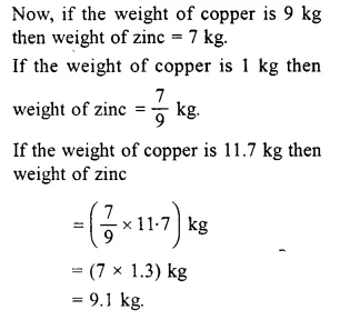
It is given that the ratio of zinc and copper in an alloy is 7 : 9.
If the weight of zinc in the alloy is 7 kg then the weight of copper in the alloy is 9 kg.
RS Aggarwal Class 6 Solutions Chapter 10 Ratio, Proportion and Unitary Method Ex 10A Q17.1

Question 18.
Solution:
A bus covers in 2 hours = 128 km
128 It will cover in 1 hour = \(\\ \frac { 128 }{ 2 } \) = 64 km
A train cover in 3 hours = 240 km
It will cover in 1 hour = \(\\ \frac { 240 }{ 3 } \)
= 80 km
Ratio in their speeds = 64: 80
= 4 : 5
{Dividing by 16, the LCM of 64, 80}

Question 19.
Solution:
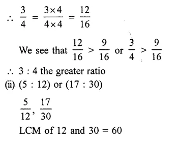
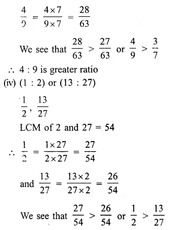
(i) (3 : 4) or (9 : 16)
LCM of 4, 16 = 16
RS Aggarwal Class 6 Solutions Chapter 10 Ratio, Proportion and Unitary Method Ex 10A Q18.1
RS Aggarwal Class 6 Solutions Chapter 10 Ratio, Proportion and Unitary Method Ex 10A Q18.2
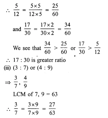
RS Aggarwal Class 6 Solutions Chapter 10 Ratio, Proportion and Unitary Method Ex 10A Q18.3
RS Aggarwal Class 6 Solutions Chapter 10 Ratio, Proportion and Unitary Method Ex 10A Q18.4

Question 20.
Solution:
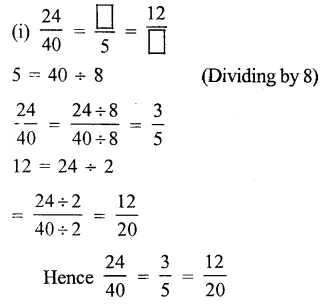
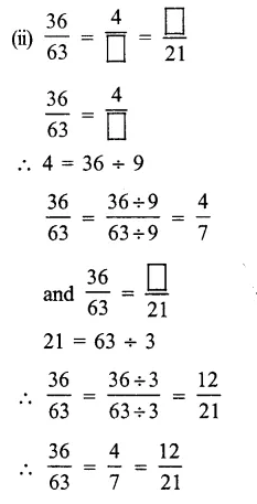
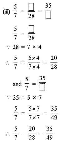
RS Aggarwal Class 6 Solutions Chapter 10 Ratio, Proportion and Unitary Method Ex 10A Q20.1
RS Aggarwal Class 6 Solutions Chapter 10 Ratio, Proportion and Unitary Method Ex 10A Q20.2
RS Aggarwal Class 6 Solutions Chapter 10 Ratio, Proportion and Unitary Method Ex 10A Q20.3


Hope given RS Aggarwal Solutions Class 6 Chapter 10 Ratio, Proportion and Unitary Method Ex 10A are helpful to complete your math homework.

If you have any doubts, please comment below. Learn Insta try to provide online math tutoring for you.

RD Sharma Class 8 Solutions Chapter 6 Algebraic Expressions and Identities Ex 6.4

RD Sharma Class 8 Solutions Chapter 6 Algebraic Expressions and Identities Ex 6.4

These Solutions are part of RD Sharma Class 8 Solutions. Here we have given RD Sharma Class 8 Solutions Chapter 6 Algebraic Expressions and Identities Ex 6.4

Other Exercises

Find the following products 

Question 1.
2a3 (3a + 5b)
Solution:
2a3 (3a + 5b) = 2a3 x 3a + 2a3 x 5b
= 6a3 +1 + 10a3b
= 6a4 + 10a3b

Question 2.
-11a (3a + 2b)
Solution:
-11a (3a + 2b) = -11a x 3a – 11a x 2b
= -33a2– 22ab

Question 3.
-5a (7a – 2b)
Solution:
-5a (7a – 2b) = -5a x 7a- 5a x (-2b)
= -35a2 + 10ab

Question 4.
-11y2 (3y + 7)
Solution:
-11y2 (3y + 7) = -11y2 x 3y – 11y2 x 7
= -33y2+1-77y2
= 33y3-77y2

Question 5.
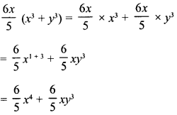
\(\frac { 6x }{ 5 }\) (x3+y3)
Solution:
RD Sharma Class 8 Solutions Chapter 6 Algebraic Expressions and Identities Ex 6.4 1

Question 6.
xy (x3-y3)
Solution:
xy (x3 – y3) =xy x x3 – xy x y3
= x1 + 3 x y – x x y1+3
= x4y – xy4

Question 7.
0.1y (0.1x5 + 0.1y)
Solution:
0.1y (0.1x5 + 0.1y) = 0.1y x 0.1x5 + 0.1y x 0.1y
= 0.01x5y + 0.01y2

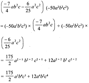
Question 8.
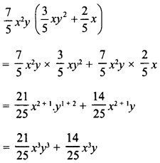
RD Sharma Class 8 Solutions Chapter 6 Algebraic Expressions and Identities Ex 6.4 2
Solution:
RD Sharma Class 8 Solutions Chapter 6 Algebraic Expressions and Identities Ex 6.4 3

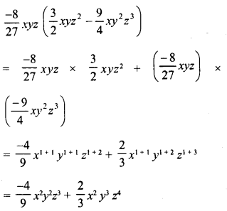
Question 9.
RD Sharma Class 8 Solutions Chapter 6 Algebraic Expressions and Identities Ex 6.4 4
Solution:
RD Sharma Class 8 Solutions Chapter 6 Algebraic Expressions and Identities Ex 6.4 5

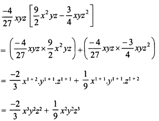
Question 10.
RD Sharma Class 8 Solutions Chapter 6 Algebraic Expressions and Identities Ex 6.4 6
Solution:
RD Sharma Class 8 Solutions Chapter 6 Algebraic Expressions and Identities Ex 6.4 7

Question 11.
5x (10x2y – 100xy2)
Solution:
5x (10x2y – 100xy2)
= 1.5x x 10x2y – 1.5x x 100xy2
= 15x1 + 2y- 150x1+1 x y2
15 x3y- 150xy2

Question 12.
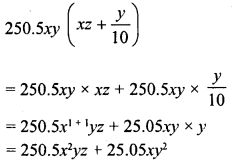
4.1xy (1.1x-y)
Solution:
4.1xy (1.1x-y) = 4.1xy x 1.1x – 4.1xy x y
= 4.51x2y-4.1xy2

Question 13.
RD Sharma Class 8 Solutions Chapter 6 Algebraic Expressions and Identities Ex 6.4 8
Solution:
RD Sharma Class 8 Solutions Chapter 6 Algebraic Expressions and Identities Ex 6.4 9

Question 14.
RD Sharma Class 8 Solutions Chapter 6 Algebraic Expressions and Identities Ex 6.4 10
Solution:
RD Sharma Class 8 Solutions Chapter 6 Algebraic Expressions and Identities Ex 6.4 11

Question 15.
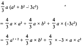
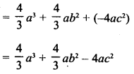
\(\frac { 4 }{ 3 }\) a (a2 + 62 – 3c2)
Solution:
RD Sharma Class 8 Solutions Chapter 6 Algebraic Expressions and Identities Ex 6.4 12
RD Sharma Class 8 Solutions Chapter 6 Algebraic Expressions and Identities Ex 6.4 13

Question 16.
Find the product 24x2 (1 – 2x) and evaluate its value for x = 3.
Solution:
24x2 (1 – 2x) = 24x2 x 1 + 24x2 x (-2x)
= 24x2 + (-48x2+1)
= 24x2 – 48x3
If x = 3, then
= 24 (3)2 – 48 (3)3
= 24 x 9-48 x 27 = 216- 1296
= -1080

Question 17.
Find the product of -3y (xy +y2) and find its value for x = 4, and y = 5.
Solution:
-3y (xy + y2) = -3y x xy – 3y x y2
= -3xy2 -3y2 +1  = -3xy2 – 3y3
If x = 4, y = 5, then
= -3 x 4 (5)2 – 3 (5)3 = -12 x 25 – 3 x 125
= -300 – 375 = – 675

Question 18.
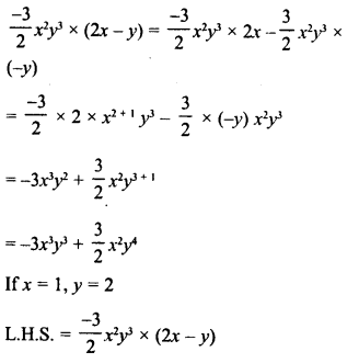
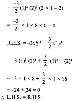
Multiply – \(\frac { 3 }{ 2 }\) x2y3 by (2x-y) and verify the answer for x = 1 and y = 2.
Solution:
RD Sharma Class 8 Solutions Chapter 6 Algebraic Expressions and Identities Ex 6.4 14
RD Sharma Class 8 Solutions Chapter 6 Algebraic Expressions and Identities Ex 6.4 15

Question 19.
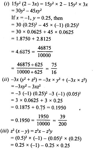
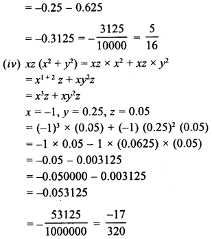
Multiply the monomial by the binomial and find the value of each for x = -1, y = 25 and z =05 :
(i) 15y2 (2 – 3x)
(ii) -3x (y2 + z2)
(iii) z2 (x – y)
(iv) xz (x2 + y2)
Solution:
RD Sharma Class 8 Solutions Chapter 6 Algebraic Expressions and Identities Ex 6.4 16
RD Sharma Class 8 Solutions Chapter 6 Algebraic Expressions and Identities Ex 6.4 17

Question 20.
Simplify :
(i) 2x2 (at1 – x) – 3x (x4 + 2x) -2 (x4 – 3x2)
(ii) x3y (x2 – 2x) + 2xy (x3 – x4)
(iii) 3a2 + 2 (a + 2) – 3a (2a + 1)
(iv) x (x + 4) + 3x (2x2 – 1) + 4x2 + 4
(v) a (b-c) – b (c – a) – c (a – b)
(vi) a (b – c) + b (c – a) + c (a – b)
(vii) 4ab (a – b) – 6a2 (b – b2) -3b2 (2a2 – a) + 2ab (b-a)
(viii) x2 (x2 + 1) – x3 (x + 1) – x (x3 – x)
(ix) 2a2 + 3a (1 – 2a3) + a (a + 1)
(x) a2 (2a – 1) + 3a + a3 – 8
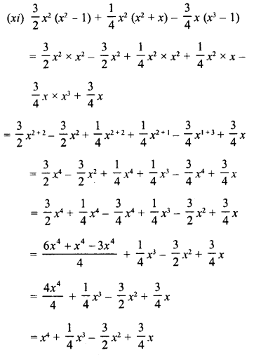
(xi) \(\frac { 3 }{ 2 }\)-x2 (x2 – 1) + \(\frac { 1 }{4 }\)-x2 (x2 + x) – \(\frac { 3 }{ 4 }\)x (x3 – 1)
(xii) a2b (a – b2) + ab2 (4ab – 2a2) – a3b (1 – 2b)
(xiii )a2b (a3 – a + 1) – ab (a4 – 2a2 + 2a) – b (a3– a2 -1)
Solution:
(i) 2x2 (x3 -x) – 3x (x4 + 2x) -2 (x4 – 3x2)
= 2xx x3-2x2x x-3x x x4-3x x 2x-2x4 + 6x2
= 2x2 + 3– 2x2 +1 – 3x,1+ 4-6x,1+1 -2x4 + 6x2
= 2x5 – 2x3 – 3x5 — 6x2 – 2x4 + 6x2
= 2x5 – 3x5 – 2a4 – 2x3 + 6x2 – 6x2
= -x5 – 2x4 – 2x3 + 0
= -x5-2x4-2x3
(ii) x3y (x2 – 2x) + 2xy (x3 – x4)
= x3y x x2 – x3y x 2x + 2ay x ac3 – 2xy x x4
= x3 + 2y-2x3 + 1 y + 2x1 + 3y – 2yx4+1
= x5y – 2x4y + 2x4y – 2yx5
= -x5y
(iii) 3a2 + 2 (a + 2) – 3a (2a + 1)
= 3a2 + 2a + 4 – 6a2 – 3a
= 3a2 – 6a2 + 2a – 3a + 4
= -3a2 – a + 4
(iv) x (x + 4) + 3x (2x2 – 1) + 4x2 + 4
= x2 + 4x + 3x x 2x2 – 3x x 1 + 4x2 + 4
= x2 + 4x + 6x2 +1 – 3x + 4x2 + 4
= x2 + 4x + 6x3 – 3x + 4x2 + 4
= 6a3 + 4x2 + x2 + 4x – 3x + 4
= 6x3 + 5x2 + x + 4
(v) a (b – c)-b (c – a) – c (a – b)
= ab – ac – be + ab – ac + bc
= 2ab – 2ac
(vi) a (b – c) + b (c – a) + c (a – b)
= ab – ac + bc – ab + ac – bc
= ab – ab + bc – be + ac – ac
= 0
(vii) 4ab (a – b) – 6a2 (b – b2) -3b2 (2a2 – a) + 2ab (b – a)
= 4a2b – 4ab2 – 6a2b + 6a2b2 – 6a2b2 + 3ab2 + 2ab2 – 2a2b
= 4a2b- 6a2b – 2 a2b – 4ab2 + 3 ab2 + 2ab2 + 6a2b2 – 6a2b2
= 4a2b – 8a2b – 4ab2 + 5 ab2 + 0
= – 4a2b + ab2
(viii) x2 (x2 + 1) – x3 (x + 1) – x (x3 – x)
= x2 + 2 + x2 – x3 + 1 – x3 – x1 + 3 + x1 + 1
= x4 + x2-x4-x3-x4 + x2
= x4-x4-x4-x3 + x2 + x2
= -x4 – x3 + 2x2
(ix) 2a2 + 3a (1 – 2a3) + a (a + 1)
= 2a2 + 3 a – 3 a x 2a3 + a2 + a
= 2a2 + 3a – 6a1 + 3 + a2 + a
= 2a2 + 3a – 6a4 + a2 + a
= -6a4 + 3a2 + 4a
(x) a2 (2a – 1) + 3a + a3 – 8
= 2 a2 x a – a2 x 1+3a + a3-8
= 2a3 – a2 + 3a + a3 – 8
= 2a3 + a3 – a2 + 3a – 8
= 3a3 – a2 + 3a – 8
RD Sharma Class 8 Solutions Chapter 6 Algebraic Expressions and Identities Ex 6.4 18
(xii) a2b (a – b2) + ab2 (4ab – 2a2) – a3b (1 – 2b)
= a2b x a – a2b x b1 + ab2 x 4ab – ab1 x2a2 -a3b x 1 + a3b x 2b
= a2+1 b-a2b2 +1+ 4a1 +1 b2 +1 -2a2+1 b2-a3b + 2a3b1 +1
= a’b – a2b3 + 4a2b3 – 2a3b2 – a3b + 2a3b2
= a3b – a3b – a2b3 + 4a2b3 – 2a3b2 + 2a3b2
= 0 + 3a2b3 + 0 = 3 a2b3
(xiii) a2b (a3 – a + 1) – ab (a4 – 2a2 + 2a) – b (a3 -a2– 1)
= a2b x a3 – a2b x a + a2b – ab x a2 + ab x 2a2 – ab x 2a- ba3 + ba2 + b
= a2+ 3b – a2+1 b + a2b -a1 + 4b + 2a1 + 2b- 2a1+1 b- a3b + a2b + b
= a5b – a3b + a26 – a5b + 2a3b – 2a2b – a3b + a2b + b
= a5b – a3b + 2a3b – a36 – a3b + a2b – 2a2b + a2b + b
= a3b – a5b + 2a3b – 2a3b + 2a2b-2a2b + b
= 0 + 0 + 0 + b = b

Hope given RD Sharma Class 8 Solutions Chapter 6 Algebraic Expressions and Identities Ex 6.4 are helpful to complete your math homework.

If you have any doubts, please comment below. Learn Insta try to provide online math tutoring for you.

CA Foundation Business Economics Study Material – Internal and External Economies

CA Foundation Business Economics Study Material Chapter 3 Theory of Production and Cost – Internal and External Economies

Internal Economies and Diseconomies

  • Internal economies are those benefits which accrue to a firm when it expands the scale of production.
  • Internal economies are the result of the firm’s own efforts independent of the actions of other firms.
  • These economies are particular to the individual firms and are different for different firms depending upon the size of the firm.

The main types of internal economies are as follows

1. Technical Economies:

– The large scale production is associated with technical economies.
– As the firm increases its scale of production, it becomes possible to use better plant, machinery, equipment and techniques of production.
– Following are the main forms (causes/reasons) of technical economies

  • Economies of superior techniques
    – A large sized firm can use sophisticated and costly machines and equipments.
    – Use of superior techniques reduces the cost of production per unit and increases aggregate output.
  • Economies of increased dimensions
    – A large firm can get the mechanical advantage in using large machines and other mechanical units to produce more output.
    – E.g. A Large boiler, large furnace, etc. can be operated by same team as required by smaller boiler, furnace, etc.
  • Economies of linked processes
    – A large sized firm can develop its own sources of raw material, means of transportation, distribution system, etc.
  • Economies of the use of By-products
    – A large sized firm can avoid all kinds of wastage of materials. The firm can use its by- products and waste material to produce another material.
    – E.g.- Sugar industry can make alcohol out of the molasses.
  • Economies of specialization
    – A large sized firm can introduce greater degree of division of labour and specialisation.

2. Managerial Economies:

  • Large sized firms can introduce division of labour in managerial tasks.
  • They can employ business executive of high skill and qualification to look after the functioning of various departments like production, finance, sales, advertising, personnel, etc.
  • This helps to increase the efficiency and productivity of managers resulting in reduction in managerial costs.

3. Commercial Economies:

  • A large sized firm is able to reap economies of bulk purchases.
  • It can get discounts from suppliers, railways, transport companies, etc.
  • It enjoys prompt and regular supply of raw materials.
  • A large sized firm can also afford to spend large amount of money on advertising, publicity, etc.
  • It can also give various concessions to wholesale and retail dealers and customers and thus capture markets for its product.

4. Financial Economies:

  • A big firm enjoys goodwill among lenders or investors.
  • For raising finance it can either borrow from bank as it can offer better security or it can raise finance by issuing shares, debentures and by inviting public deposits. Such opportunities are not available to small firms.

5. Risk Bearing Economies:

  • A large firm is better placed to face the uncertainties and risks of business.
  • A big firm producing many variety of goods is in a better position to withstand economic ups and downs. Therefore, it enjoys economies of risk bearing.

Internal diseconomies means all those factors which raise the cost of production per unit of a particular firm when the scale of production is expanded beyond the point of optimal capacity.

Such diseconomies of scale are as follows

1. Production Diseconomies:

  • Production diseconomies sets in when expansion of firm’s production beyond optimum size leads to rise in the cost per unit of output.
  • E.g. Use of inferior or less efficient factors due to non-availability of efficient factors raises the per unit cost of output.

2. Managerial Diseconomies:

  • As the scale of production increases burden on management also increases.
  • Co-ordination of work among different departments becomes difficult. Supervision and control over the activities of subordinates becomes difficult, decision taking is delayed, etc.
  • As a result, wastage increase and the efficiency and productivity decrease.
  • Per unit cost starts rising.

3. Technical Diseconomies:

  • Every equipment has an optimum point at which it works more efficiently and economically.
  • Beyond optimum point they are overworked and may result in breakdowns, heavy cost of maintenance, etc.

4. Financial Diseconomies:

  • Expansion of production beyond the optimum scale results in increase in the cost of capital.
  • It may be due to increased dependence on external finances.

5. Marketing Diseconomies:

  • Selling diseconomies set in if the scale of production is expanded beyond optimum level.
  • The advertisement expenditure and marketing overheads increase more proportionately with the scale.

External Economies and Diseconomies

  • External economies are those benefits which accrue to all the firms operating in a given industry from the growth and expansion of that industry.
  • External economies are not related to an individual firm’s own cost reduction efforts.
  • These are common to all the firms in an industry and shared by many firms or industries.

The main types of external economies are as follows

1. Technological Economies:

  • When the whole industry expands, it may result in the discovery of new technical knowledge, firms pool manpower and finance for research and development resulting in new and improved methods of production and new inventions.
  • Use of improved and better machinery improves production function and cost of production per unit falls.

2. Economies of Localization:

  • When in an area, many firms producing the same commodity are set up, it is called localization of an industry.
  • Due to localization there is expansion of railways, post & telegraph, banking services, insurance, setting up of booking offices by transport, companies, setting § up of powerful transformer by electricity department, etc.
  • All the firms get these facilities at low prices.

3. Economies of Information:

  • As pointed earlier, firms pool their resources for research and development.
  • All firms get the benefit of the research in terms of market information, technical information, information about governments economic policies, information about availability of new source of raw material, etc.
  • Also, specialized journals give information about latest developments.

4. Cheaper Inputs:

  • When an industry expands its needs for raw materials, machines, etc. also expand.
  • This may result in exploration of new and cheaper sources of raw materials, machinery, etc.
  • Also, the industries producing such inputs also expand in scale.
  • Therefore, they can supply these inputs at lower prices.
  • As a result the cost of production per unit of the firm using these inputs falls.

5. Growth of Ancillary Industries:

  • With the growth of an industry, many firms specialized in the production of inputs like raw material, tools, machinery, etc. come up.
  • Such firms are called ancillary units which provides inputs at lower cost to the main industry.
  • Likewise, some firms may get developed by processing the waste products of the industry.
  • Thus, wastes are converted into by-products. This reduces the cost of production in general.

6. Development of Skilled Labour:

  • When an industry expands specialized institutions like colleges, training centers, management institutes, etc. develop.
  • This results in continuous availability of skilled labour like technicians, engineers, management experts, etc.

7. Better transportation & Marketing Facilities:-

  • When an industry expands many specialized transporters also develop.
  • The firm in need of specialized transport service can get them easily at cheaper rates.
  • Also many new marketing outlets and specialized marketing institutions develop. The firm need not spend on developing its own marketing outlets.
  • This reduces the cost.

The growth and expansion of an industry in a particular area beyond optimum level results in many disadvantages for firms in the industry. Such disadvantages increases the costs of production of each firm. Therefore, they are called external diseconomies. Some of the external diseconomies are as follows:

1. Diseconomies of Scarcity of Inputs:

  • When an industry expands its need for raw materials, machines, tools and equipments, etc. also expands.
  • Some inputs are such which cannot be totally substituted.
  • The firms supplying these inputs come under pressure and may supply inputs at a higher price.
  • This raises the cost of production per unit of the firm who uses these inputs.

2. Diseconomies of Strains on Infrastructure:

  • Due to concentration of firms in an area infrastructural facilities become inadequate over a time.
  • E.g. Excessive pressure on transport system results in delayed transportation of raw materials and finished goods.
  • Other facilities like electric power supply, communication system, water supply, etc. are also over taxed.
  • This puts strain on infrastructural facilities resulting in increased cost of production. ’

3. Diseconomies of High Factor Prices:

  • With the concentration of an industry in a particular area, the demand for factors of production rises.
  • Thus, the prices of the factors of production go up resulting in increased cost of production.

4. Diseconomies of Expenditure on Advertising:

  • Expansion of an industry also means increase in the number of firms.
  • This means increase in competition among the firms.
  • This forces a firm to spend more and more on advertising.
  • This raises per unit cost.

Internal and External Economies

S.NoINTERNAL ECONOMIESEXTERNAL ECONOMIES
1.
  • Internal economies are the benefits which accrue to a firm when it expands the scale of production.
  • External economies are those benefits which accrue to all the firms operating in a given industry from the growth and expansion of that industry.
2.
  • Internal economies are called ‘internal’ because these arise due to the internal efforts of the firm.
  • These economies are specific to the individual firm and are different for different firms depending upon the size of the firm.
  • External economies are called ‘external’ because they accrue to a firm as a result of factors that are entirely outside the firm i.e. from the expansion of the industry.
3.
  • Internal economies are the result of the firm’s OWN EFFORTS INDEPENDENT OF THE ACTIONS OF OTHER FIRMS.
  • These economies are peculiar to each fir m.
  • It reflects the working pattern of the firm.
  • External economies are independent of firm’s own efforts and output.
  • They are dependent on the general development of the industry.
  • They are not restricted to a single firm but are shared by a number of firms.
4.
  • Internal economies cause the long-run average cost to fall in the initial stage and internal diseconomies cause the long-run average cost to rise at the later stage.
  • Thus, the shape of LAC curve is determined by internal economies and diseconomies as scale expands.
  • External economies and diseconomies cause the LAC curve to shift down or up as the case may be.
  • When external economies increase, the cost per unit of output falls.
  • So, LAC curve shift downwards.
  • When external diseconomies are more, the cost per unit of output rises.
  • So, LAC curve shift upwards.
5.CA Foundation Business Economics Study Material Internal and External Economies 1CA Foundation Business Economics Study Material Internal and External Economies 2
6.
  • If every thing is effectively managed, internal economies can be of long term in nature.
  • External economies depend upon the conditions of the entire industry and economy.
  • Thus, it can be of short term in nature.
7.
  • Internal economies are in the form of technical economies like superior techniques, use of by- products, etc.; managerial economies; commercial economies; financial economies and risk-bearing economies.
  • External economies are in the form of cheaper inputs; discovery of new technical knowledge; development of skilled labour; economies of information; growth of ancillary units; better transport and marketing facilities.

CA Foundation Business Economics Study Material – Production Optimisation

CA Foundation Business Economics Study Material Chapter 3 Theory of Production and Cost – Production Optimisation

Production Optimisation
Isoquants:

An iso-product curve or isoquant is a curve, which represents the various combinations of two variable inputs that give the same level of output. As all combinations on the iso-product curve give the same level of output, the producer becomes indifferent to these combinations. That is why iso-product curve are also called ‘production indifference curve’ or ‘equal product curve’. To understand consider the following production isoquant schedule.

CA Foundation Business Economics Study Material Production Optimisation 1

In the schedule I above, the producer is indifferent whether he gets combination A, B, C, D or E. This is because all the combinations of capital and labour give the same level of output i.e. 100 units.

By plotting the above combinations on a graph, we can derive an iso-product curve as shown in the following figure:

CA Foundation Business Economics Study Material Production Optimisation 2

In the diagram, quantity of capital is measured on X-axis and quantity of labour on Y-axis.

The various combinations A, B, C, D, E of capital and labour are plotted and on joining them we derive an iso-product curve. All combinations lying on the iso-product curve yield the same level of output i.e. 100 units and hence technically equally efficient.

If the production schedule II is also plotted on the graph, we will get another iso-product curve IQ200. This will lie above the IQ100 as the combinations contain greater quantities of capital and labour. A set of iso-product curves is called iso-product curve map.

CA Foundation Business Economics Study Material Production Optimisation 3

In the diagram, it can be observed that each iso-product curve is labelled in terms of output. All combinations lying of IQ100 give the output of 100 units and all the combinations lying on IQ200 give the output of 200 units. Higher iso-product curve represent higher level of output. Also it indicates how much more output can be achieved.

Marginal Rate of Technical Substitution
The rate at which one factor of production is substituted in place of the other factor without any change in the level of output is called as the marginal rate of technical substitution. Consider the following schedule.

CA Foundation Business Economics Study Material Production Optimisation 4

Each of the factor combinations in the table above yields same level of output. Moving from combination A to B, one unit of capital replaces 4 units of labour. Similarly, moving from B to C, one unit of capital now replaces only 3 units of labour and so on. It implies that labour and capital are imperfect substitutes. That is why MRTSKL is continuously diminishing. We can measure MRTSKL on an iso-product curve.

‘Iso-Cost Line’ OR ‘Equal Cost Lines’
Iso-cost line (also known Equal Cost Line; Price Line; Outlay Line; Factor Price Line) shows the various combinations of two factor inputs which the firm can purchase with a given outlay (i.e. budget) and at given prices of two inputs.

Example. A firm has with itself Rs. 1,000 which it would like to spend on factor ‘X’ and factor ‘Y’.
Price of factor ‘X’ is Rs. 20 per unit.
Price of factor ‘Y’ is Rs. 10 per unit.
Therefore, if the firm spends the whole amount on factor X, it can buy 50 units of X and if the whole amount is spent on factor Y, it can buy 100 units of Y. However, in between these two extreme limits, it can have many combinations of X and Y for the outlay of Rs. 1,000. Graphically it can be shown as follows –

CA Foundation Business Economics Study Material Production Optimisation 5

In the diagram OP shows 100 units of Y and OM shows 50 units of X. When we join the two points P and M, we get the iso-cost line. All the combinations of factor X and factor Y lying on iso-cost line can be purchased by the firm with an outlay of Rs. 1,000. If the firm increases the outlay to Rs. 2,000, the iso-cost line shifts to the right, if prices of two factors remains unchanged. The slope of the iso-cost line is equal to the ratio of the prices of two factors. Thus,
CA Foundation Business Economics Study Material Production Optimisation 6

Producer’s Equilibrium OR Production Optimization
A firm always try to produce a given level of output at minimum cost. For this it has to use that combination of inputs which minimizes the cost of production. This ensures maximization of profits and produce a given level of output with least cost combination of inputs. The least-cost combination of inputs or factors is called producer’s equilibrium or production optimization. This is determined with the help of (a) isoquants, & (b) iso-cost line.

An isoquant or iso-product curve is a curve which shows the various combinations of two inputs that produce same level of output. The isoquants are negatively sloped and convex to origin. The slope of isoquants shows the marginal rate of technical substitution which diminishes. Thus, MRTSxy
CA Foundation Business Economics Study Material Production Optimisation 7
Iso-cost line shows the various combination of two factor inputs which the firm can purchase with a given outlay and at given prices of inputs. There can be different outlays and hence different iso-cost lines. Slope of iso-cost line shows the ratio of the price of two inputs i.e. Px/Py

CA Foundation Business Economics Study Material Production Optimisation 8

Which will be the least cost combination can be understood with the help of following figure. Suppose firm wants to produce 300 units of a commodity. It will first see the isoquant that represents 300 units.

In the adjoining diagram we find that all combinations a, b, c, d and e can produce 300 units of output. In order to produce 300 units firm with try to find out least cost combination. For this it will super impose the various iso-cost lines on isoquant as shown in the diagram. The diagram shows that combination ‘C’ is,the least cost combination as here isoquant is tangent to iso-cost line HI. All other combinations a, b, d and e lying on isoquant cost more as these points lie on higher iso-cost lines. Hence, the point of tangency of isoquant and iso-cost line shows least cost combination. At the point of tangency.

Slope of iso-quant = Slope of iso-cost line

CA Foundation Business Economics Study Material Production Optimisation 9
Thus, the firm will choose OM units of factor X and ON units of factor Y and be at equilibrium as the marginal physical products of two factors are proportional to the factor prices.