Prasanna

Find free online Chemistry Topics covering a broad range of concepts from research institutes around the world.

Nomenclature of Elements with Atomic Number Greater than 100

Usually, when a new element is discovered, the discoverer suggests a name following IUPAC guidelines which will be approved after a public opinion. In the meantime, the new element will be called by a temporary name coined using the following IUPAC rules, until the IUPAC recognises the new name.

1. The name was derived directly from the atomic number of the new element using the following numerical roots.

Notation for IUPAC Nomenclature of Elements

2. The numerical roots corresponding to the atomic number are put together and ‘ium’ is added as suffix

3. The final ‘n’ of ‘enn’ is omitted when it is written before ‘nil’ (enn + nil = enil) similarly the final ‘i’ of ‘bi’ and ‘tri’ is omitted when it written before ‘ium’ (bi + ium = bium; tri + ium = trium)

4. The symbol of the new element is derived from the first letter of the numerical roots.

The following table illustrates these facts.

To overcome all these difficulties, IUPAC nomenclature has been recommended for all the elements with Z > 100. It was decided by IUPAC that the names of elements beyond atomic number 100 should use Latin words for their numbers. The names of these elements are derived from their numerical roots.

Fermium is a synthetic element with the symbol Fm and atomic number 100. It is an actinide and the heaviest element that can be formed by neutron bombardment of lighter elements, and hence the last element that can be prepared in macroscopic quantities, although pure fermium metal has not yet been prepared.

The twelve elements of nature are Earth, Water, Wind, Fire, Thunder, Ice, Force, Time, Flower, Shadow, Light and Moon.

Uranium

The heaviest element known to occur in nature is uranium, which contains only 92 protons, putting it 30 places below the putative new element in the periodic table. In the laboratory, physicists have managed to create elements up to 118, but they are all highly unstable.

The fifth element on top of earth, air, fire, and water, is space or aether. It was hard for people to believe that the stars and everything else in space were made of the other elements, so space was considered as a fifth element.

According to ancient and medieval science, aether also spelled ether, aither, or ether and also called quintessence (fifth element), is the material that fills the region of the universe above the terrestrial sphere.

Find free online Chemistry Topics covering a broad range of concepts from research institutes around the world.

Moseley’s Work and Modern Periodic Law

In 1913, Henry Moseley studied the characteristic X-rays spectra of several elements by bombarding them with high energy electrons and observed a linear correlation between atomic number and the frequency of X-rays emitted which is given by the following expression.

\(\sqrt{υ}\) = a(Z – b)

Where, υ is the frequency of the X-rays emitted by the element with atomic number ‘Z’; a and b are constants and have same values for all the elements.

The plot of \(\sqrt{υ}\) against Z gives a straight line. Using this relationship, we can determine the atomic number of an unknown (new) element from the frequency of X-ray emitted. Based on his work, the modern periodic law was developed which states that, “the physical and chemical properties of the elements are periodic functions of their atomic numbers.” Based on this law, the elements were arranged in order of their increasing atomic numbers.

This mode of arrangement reveals an important truth that the elements with similar properties recur after regular intervals. The repetition of physical and chemical properties at regular intervals is called periodicity.

Modern Periodic Table

The physical and chemical properties of the elements are correlated to the arrangement of electrons in their outermost shell (valence shell). Different elements having similar outer shell electronic configuration possess similar properties. For example, elements having one electron in their valence shell s-orbital possess similar physical and chemical properties. These elements are grouped together in the modern periodic table as first group elements.

Similarly, all the elements are arranged in the modern periodic table which contains 18 vertical columns and 7 horizontal rows. The vertical columns are called groups and the horizontal rows are called periods. Groups are numbered 1 to 18 in accordance with the IUPAC recommendation which replaces the old numbering scheme IA to VIIA, IB to VIIB and VIII.

Each period starts with the element having general outer electronic configuration ns¹ and ends with ns² np⁶.
Here ‘n’ corresponds to the period number (principal quantum number). The aufbau principle and the  electronic configuration of atoms provide a theoretical foundation for the modern periodic table.

Find free online Chemistry Topics covering a broad range of concepts from research institutes around the world.

Classification of Elements

During the 19^th century, scientists have isolated several elements and the list of known elements increased. Currently, we have 118 known elements. Out of 118 elements, 92 elements with atomic numbers 1 to 92 are found in nature. Scientists have found out there are some similarities in properties among certain elements.

This observation has led to the idea of classification of elements based on their properties. In fact, classification will be beneficial for the effective utilization of these elements. Several attempts were made to classify the elements. However, classification based on the atomic weights led to the construction of a proper form of periodic table.

In 1817, J. W. Dobereiner classified some elements such as chlorine, bromine and iodine with similar chemical properties into the group of three elements called as triads. In triads, the atomic weight of the middle element nearly equal to the arithmetic mean of the atomic weights of the remaining two elements. However, only a limited number of elements can be grouped as triads.

This concept can not be extended to some triads which have nearly same atomic masses such as [Fe, Co, Ni], [Ru, Rh, Pd] and [Os, Ir, Pt].

In 1862, A. E. B. de Chancourtois reported a correlation between the properties of the elements and their atomic weights. He said ‘the properties of bodies are the properties of numbers’. He intended the term numbers to mean the value of atomic weights.

He designed a helix by tracing at an angle 45˚ to the vertical axis of a cylinder with circumference of 16 units. He arranged the elements in the increasing atomic weights along the helix on the surface of this cylinder.

One complete turn of a helix corresponds to an atomic weight increase of 16. Elements which lie on the 16 equidistant vertical lines drawn on the surface of cylinder shows similar properties. This was the first reasonable attempt towards the creation of periodic table. However, it did not attract much attention.

In 1864, J. Newland made an attempt to classify the elements and proposed the law of octaves. On arranging the elements in the increasing order of atomic weights, he observed that the properties of every eighth element are similar to the properties of the first element. This law holds good for lighter elements up to calcium.

Mendeleev’s Classification

In 1868, Lothar Meyer had developed a table of the elements that closely resembles the modern periodic table. He plotted the physical properties such as atomic volume, melting point and boiling point against atomic weight and observed a periodical pattern.

During same period Dmitri Mendeleev independently proposed that “the properties of the elements are the periodic functions of their atomic weights” and this is called periodic law. Mendeleev listed 70 elements, which were known till histime in several vertical columns in order of increasing atomic weights. Thus, Mendeleev constructed the first periodic table based on the periodic law.

As shown in the periodic table, he left some blank spaces since there were no known elements with the appropriate properties at that time. He and others predicted the physical and chemical properties of the missing elements. Eventually these missing elements were discovered and found to have the predicted properties.

For example, Gallium (Ga) of group III and germanium (Ge) of group IV were unknown at that time. But Mendeleev predicted their existence and properties. He referred the predicted elements as eka-aluminium and eka-silicon. After discovery of the actual elements, their properties were found to match closely to those predicted by Mendeleev (Table 3.4).

Properties predicted for Eka-aluminium and Eka-silicon

Anomalies of Mendeleev’s Periodic Table

Some elements with similar properties were placed in different groups and those with dissimilar properties were placed in same group. Similarly elements with higher atomic weights were placed before lower atomic weights based on their properties in contradiction to his periodic law. Example ⁵⁹Co₂₇ was placed before ^58.7Ni₂₈; Tellurium (127.6) was placed in VI group but Iodine (127.0) was placed in VII group.

Find free online Chemistry Topics covering a broad range of concepts from research institutes around the world.

Filling of Orbitals

In an atom, the electrons are filled in various orbitals according to aufbau principle, Pauli exclusion principle and Hund’s rule. These rules are described below.

Aufbau Principle:

The word Aufbau in German means ‘building up’. In the ground state of the atoms, the orbitals are filled in the order of their increasing energies. That is the electrons first occupy the lowest energy orbital available to them.

Once the lower energy orbitals are completely filled, then the electrons enter the next higher energy orbitals. The order of filling of various orbitals as per the Aufbau principle is given in the figure 2.12 which is in accordance with (n+ l) rule.

Pauli Exclusion Principle:

Pauli formulated the exclusion principle which states that “No two electrons in an atom can have the same set of values of all four quantum numbers.”

It means that, each electron must have unique values for the four quantum numbers (n, l, m and s). For the lone electron present in hydrogen atom, the four quantum numbers are: n = 1; l = 0; m = 0 and s = + ½. For the two electrons present in helium, one electron has the quantum numbers same as the electron of hydrogen atom, n = 1, l = 0, m = 0 and s = + ½. For other electron, the fourth quantum number is different i.e., n = 1, l = 0, m = 0 and s = – ½.

As we know that the spin quantum number can have only two values + ½ and – ½, only two electrons can be accommodated in a given orbital in accordance with Pauli exclusion principle. Let us understand this by writing all the four quantum numbers for the eight electron in L shell.

Hund’s Rule of Maximum Multiplicity

The Aufbau principle describes how the electrons are filled in various orbitals. But the rule does not deal with the filling of electrons in the degenerate orbitals (i.e. orbitals having same energy) such as p_x, p_y, p_z. In what order these orbitals to be filled? The answer is provided by the Hund’s rule of maximum multiplicity. It states that electron pairing in the degenerate orbitals does not take place until all the available orbitals contains
one electron each.

We know that there are three p orbitals, five d orbitals and seven f orbitals. According to this rule, pairing of electrons in these orbitals starts only when the 4^th, 6^th and 8^th electron enters the p, d and f orbitals respectively.

For example, consider the carbon atom which has six electrons. According to Aufbau principle, the electronic configuration is 1s², 2s², 2p² It can be represented as below,

In this case, in order to minimise the electron-electron repulsion, the sixth electron enters the unoccupied 2p_y orbital as per Hunds rule. i.e. it does not get paired with the fifth electron already present in the 2px orbital.

Electronic Configuration of Atoms

The distribution of electrons into various orbitals of an atom is called its electronic configuration. It can be written by applying the aufbau principle, Pauli exclusion principle and Hund’s rule. The electronic configuration is written as nl^x, where n represents the principle of quantum number, ‘l’ represents the letter designation of the orbital [s(l=0), p (l=1), d(l=2) and f(l=3)] and ‘x’ represents the number of electron present in that orbital.

Let us consider the hydrogen atom which has only one electron and it occupies the lowest energy orbital i.e. 1s according to aufbau principle. In this case n = 1; l = s; x = 1.

Hence the electronic configuration is 1s¹. (read as one-ess-one).

The orbital diagram for this configuration is,

The electronic configuration and orbital diagram for the elements upto atomic number 10 are given below:

The actual electronic configuration of some elements such as chromium and copper slightly differ from the expected electronic configuration in accordance with the Aufbau principle.

For chromium – 24

Expected Configuration:

1s² 2s² 2p⁶ 3s² 3p⁶ 3d⁴ 4s²

Actual Configuration:

1s² 2s² 2p⁶ 3s² 3p⁶ 3d⁵ 4s¹

For copper – 29

Expected Configuration:

1s² 2s² 2p⁶ 3s² 3p⁶ 3d⁹ 4s²

Actual Configuration:

1s² 2s² 2p⁶ 3s² 3p⁶ 3d¹⁰ 4s¹

The reason for above observed configuration is that fully filled orbitals and half filled orbitals have been found to have extra stability. In other words, p³, p⁶, d⁵, d¹⁰, f⁷ and f¹⁴ configurations are more stable than p², p⁵, d⁴, d⁹, f⁶ and f¹³. Due to this stability, one of the 4s electrons occupies the 3d orbital in chromium and copper to attain the half filled and the completely filled configurations respectively.

Stability of Half filled and Completely Filled Orbitals:

The exactly half filled and completely filled orbitals have greater stability than other partially filled configurations in degenerate orbitals. This can be explained on the basis of symmetry and exchange energy. For example chromium has the electronic configuration of [Ar]3d⁵ 4s¹ and not [Ar]3d⁴ 4s² due to the symmetrical distribution and exchange energies of d electrons.

Symmetrical Distribution of Electron:

Symmetry leads to stability. The half filled and fully filled configurations have symmetrical distribution of electrons (Figure 2.13) and hence they are more stable than the unsymmetrical configurations.

The degenerate orbitals such as p_x, p_y, p_z have equal energies and their orientation in space are different
as shown in Figure 2.14. Due to this symmetrical distribution, the shielding of one electron on the other is relatively small and hence the electrons are attracted more strongly by the nucleus and it increases the stability.

Exchange Energy:

If two or more electrons with the same spin are present in degenerate orbitals, there is a possibility for exchanging their positions. During exchange process the energy is released and the released energy is called exchange energy. If more number of exchanges are possible, more exchange energy is released. More number of exchanges are possible only in case of half filled and fully filled configurations.

For example, in chromium the electronic confiuration is [Ar]3d⁵ 4s¹. The 3d orbital is half filled and there are ten possible exchanges as shown in Figure 2.15. On the other hand only six exchanges are possible for [Ar]3d⁴ 4s² configuration. Hence, exchange energy for the half filled confiuration is more. This increases the stability of half filled 3d orbitals.

The exchange energy is the basis for Hund’s rule, which allows maximum multiplicity, that is electron pairing is possible only when all the degenerate orbitals contain one electron each.

Find free online Chemistry Topics covering a broad range of concepts from research institutes around the world.

Quantum Numbers

The electron in an atom can be characterised by a set of four quantum numbers, namely principal quantum number (n), azimuthal quantum number (l), magnetic quantum number (m) and spin quantum number (s). When Schrodinger equation is solved for a wave function Ψ, the solution contains the first three quantum numbers n, l and m. The fourth quantum number arises due to the spinning of the electron about its own axis. However, classical pictures of species spinning around themselves are incorrect.

Principal Quantum Number (n):

This quantum number represents the energy level in which electron revolves around the nucleus and is denoted by the symbol ‘n’.

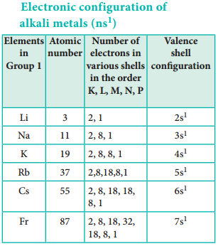
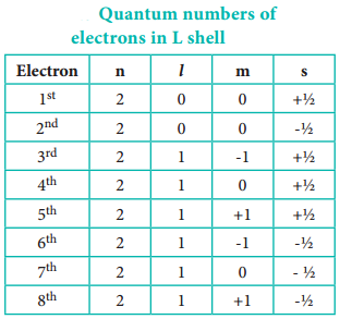
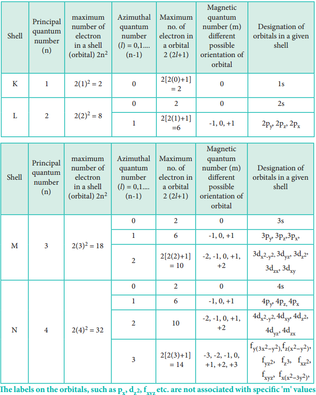
1. The ‘n’ can have the values 1, 2, 3, … n = 1 represents K shell; n = 2 represents L shell and n = 3, 4, 5 represent the M, N, O shells, respectively.

2. The maximum number of electrons that can be accommodated in a given shell is 2n².

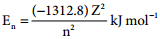
3. ‘n’ gives the energy of the electron,

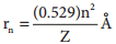
and the distance of the electron from the nucleus is given by

Azimuthal Quantum Number (l) or Subsidiary Quantum Number:

1. It is represented by the letter ‘l’, and can take integral values from zero to n-1, where n is the principal quantum number.
2. Each l value represents a subshell (orbital). l = 0, 1, 2, 3 and 4 represents the s, p, d, f and g orbitals respectively.
3. The maximum number of electrons that can be accommodated in a given subshell (orbital) is 2(2l + 1).
4. It is used to calculate the orbital angular momentum using the expression

Angular momentum = \(\sqrt{l(l+1)}\) \(\frac{h}{2π}\) …………. (2.4)

Magnetic Quantum Number (ml):

1. It is denoted by the letter ‘ml’. It takes integral values ranging from -l to +l through 0. i.e. if l = 1; m = -1, 0 and +1
2. Different values of m for a given l value, represent different orientation of orbitals in space.
3. The Zeeman Effect (the splitting of spectral lines in a magnetic field) provides the experimental justification for this quantum number.
4. The magnitude of the angular momentum is determined by the quantum number l while its direction is given by magnetic quantum number.

Spin Quantum Number (m_s):

1. The spin quantum number represents the spin of the electron and is denoted by the letter ‘m_s‘
2. The electron in an atom revolves not only around the nucleus but also spins. It is usual to write this as electron spins about its own axis either in a clockwise direction or in anti-clockwise direction.
3. The visualisation is not true. However spin is to be understood as representing a property that revealed itself in magnetic fields.
4. Corresponding to the clockwise and anti-clockwise spinning of the electron, maximum two values are possible for this quantum number.
5. The values of ‘m_s‘ is equal to -½ and + ½

Quantum Numbers and its Significance

Shapes of Atomic Orbitals:

The solution to Schrodinger equation gives the permitted energy values called eigen values and the wave functions corresponding to the eigen values are called atomic orbitals. The solution (Ψ) of the Schrodinger wave equation for one electron system like hydrogen can be represented in the following form in spherical polar coordinates r, θ, φ as,

Ψ (r, θ, φ) = R(r).f(θ).g(φ) ………….. (2.15)

(where R(r) is called radial wave function, other two functions are called angular wave functions)

As we know, the Ψ itself has no physical meaning and the square of the wave function |Ψ|² is related to the probability of finding the electrons within a given volume of space. Let us analyse how |Ψ|² varies with the distance from nucleus (radial distribution of the probability) and the direction from the nucleus (angular distribution of the probability).

Radial Distribution Function:

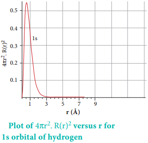
Consider a single electron of hydrogen atom in the ground state for which the quantum numbers are n = 1 and l = 0. i.e. it occupies 1s orbital. The plot of R(r)² versus r for 1s orbital is given in Figure 2.3

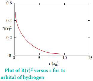
The graph shows that as the distance between the electron and the nucleus decreases, the probability of finding the electron increases. At r=0, the quantity R(r)² is maximum i.e. The maximum value for |Ψ|² is at the nucleus. However, probability of finding the electron in a given spherical shell around the nucleus is important. Let us consider the volume (dV) bounded by two spheres of radii r and r + dr.

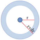
Volume of the sphere, V = \(\frac{4}{3}\)πr³
\(\frac{dV}{dr}\) = \(\frac{4}{3}\)π(3r²)
dV = \(\frac{4}{3}\)π(3r²)
dV = 4πr²dr
Ψ²dV = 4πr²Ψ²dr ……………. (2.16)

The plot of 4πr². R(r)² versus r is given below.

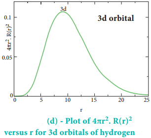
The above plot shows that the maximum probability occurs at distance of 0.52 Å from the nucleus. This is equal to the Bohr radius. It indicates that the maximum probability of finding the electron around the nucleus is at this distance. However, there is a probability to find the electron at other distances also. The radial distribution function of 2s, 3s, 3p and 3d orbitals of the hydrogen atom are represented as follows.

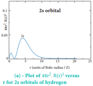
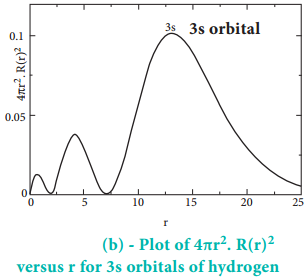
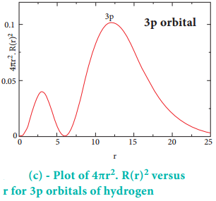
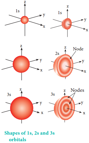
For 2s orbital, as the distance from nucleus r increases, the probability density first increases, reaches a small maximum followed by a sharp decrease to zero and then increases to another maximum, after that decreases to zero.

The region where this probability density function reduces to zero is called nodal surface or a radial node. In general, it has been found that nsorbital has (n-1) nodes. In other words, number of radial nodes for 2s orbital is one, for 3s orbital it is two and so on. The plot of 4πr². R(r)² versus r for 3p and 3d orbitals shows similar pattern but the number of radial nodes are equal to(n-l-1) (where n is principal quantum number and l is azimuthal quantum number of the orbital).

Angular Distribution Function:

The variation of the probability of locating the electron on a sphere with nucleus at its centre depends on the azimuthal quantum number of the orbital in which the electron is present. For 1s orbital, l=0 and m=0. f(θ) = 1/\(\sqrt{2}\) and g(φ) = 1/\(\sqrt{2π}\).

Therefore, the angular distribution function is equal to 1/\(\sqrt{2π}\). i.e. it is independent of the angle θ and φ. Hence, the probability of finding the electron is independent of the direction from the nucleus. The shape of the s orbital is spherical as shown in the figure 2.7.

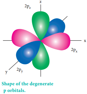
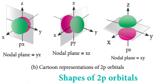
For p orbitals l = 1 and the corresponding m values are -1, 0 and +1. The angular distribution functions are quite complex and are not discussed here. The shape of the p orbital is shown in Figure 2.8. The three different m values indicates that there are three different orientations possible for p orbitals.

These orbitals are designated as p_x, p_y and p_z and the angular distribution for these orbitals shows that the lobes are along the x, y and z axis respectively. As seen in the Figure 2.8 the 2p orbitals have one nodal plane.

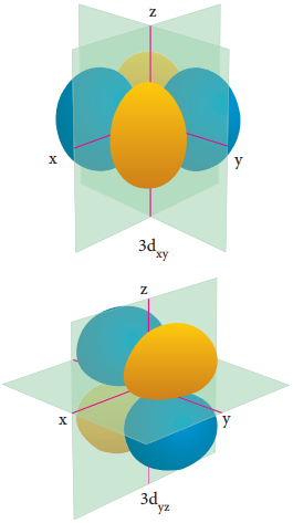
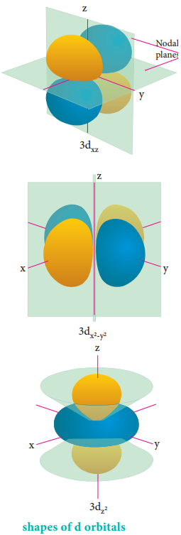
For ‘d’ orbital l = 2 and the corresponding m values are -2, -1, 0 +1,+2. The shape of the d orbital looks like a ‘clover leaf ‘. The five m values give rise to five d orbitals namely d_xy, d_yz, d_zx, d_x2-y2 and d_z2. The 3d orbitals contain two nodal planes as shown in Figure 2.9.

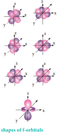
For ‘f ‘ orbital, l = 3 and the m values are -3, -2, -1, 0, +1, +2, +3 corresponding to seven f orbitals f_z³, f_xz²,
f_yz², f_xyz, f_z(x²-y²), f_x(x²-3y²), f_y(3x²-y²), which are shown in Figure 2.10. There are 3 nodal planes in the f-orbitals.

Energies of Orbitals

In hydrogen atom, only one electron is present. For such one electron system, the energy of the electron in the n^th orbit is given by the expression

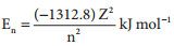
From this equation, we know that the energy depends only on the value of principal quantum number. As the n value increases the energy of the orbital also increases. The energies of various orbitals will be in the following order:

1s < 2s = 2p < 3s = 3p = 3d < 4s = 4p = 4d = 4f < 5s = 5p = 5d = 5f < 6s = 6p = 6d = 6f < 7s

The electron in the hydrogen atom occupies the 1s orbital that has the lowest energy. This state is called ground state. When this electron gains some energy, it moves to the higher energy orbitals such as 2s, 2p etc… These states are called excited states.

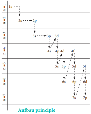
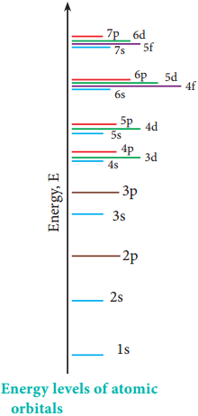
However, the above order is not true for atoms other than hydrogen (multi-electron systems). For such systems the Schrodinger equation is quite complex. For these systems the relative order of energies of various orbitals is given approximately by the (n+l) rule.

It states that, the lower the value of (n + l) for an orbital, the lower is its energy. If two orbitals have the same value of (n + l), the orbital with lower value of n will have the lower energy. Using this rule the order of energies of various orbitals can be expressed as follows.

n+ l values of different orbitals

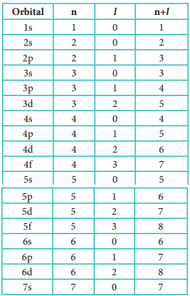
Based on the (n+ l) rule, the increasing order of energies of orbitals is as follows:

1s < 2s < 2p < 3s < 3p < 4s < 3d < 4p < 5s < 4d < 5p < 6s < 4f < 5d < 6p < 7s < 5f < 6d

As we know there are three different orientations in space that are possible for a p orbital. All the three p orbitals, namely, p_x, p_y and p_z have same energies and are called degenerate orbitals. However, in the presence of magnetic or electric field the degeneracy is lost.

In a multi-electron atom, in addition to the electrostatic attractive force between the electron and nucleus, there exists a repulsive force among the electrons. These two forces are operating in the opposite direction. This results in the decrease in the nuclear force of attraction on electron.

The net charge experienced by the electron is called effective nuclear charge. The effective nuclear charge depends on the shape of the orbitals and it decreases with increase in azimuthal quantum number l. The order of the effective nuclear charge felt by a electron in an orbital within the given shell is s > p > d > f. Greater the effective nuclear charge, greater is the stability of the orbital. Hence, within a given energy level, the energy of the orbitals are in the following order. s < p < d < f.

The energies of same orbital decrease with an increase in the atomic number. For example, the energy of the 2s orbital of hydrogen atom is greater than that of 2s orbital of lithium and that of lithium is greater than that of sodium and so on, that is, E_2s(H) > E_2s(Li) > E_2s(K).